Lessons Learned While Solving Time-Series Forecasting as a Supervised ML Problem: Part 2

In part 1 of the series, we discussed data transformation and feature engineering related learnings like missing value imputations, sliding window transform, date features, and descriptive features using history data. In this part, we will focus on approaches to be followed while creating an ML model and making predictions.

Time-series forecasting problems can be classified into two broad categories based on the number of time-steps to be forecasted.

• One-step Forecasting: Only next time period value to be forecasted like monthly sales in October based on monthly sales time-series till September or next day stock prices based on daily stock prices till today
• Multi-step Forecasting: More than one future time-periods to be forecasted like monthly sales in October, November, and December using monthly sales till September or next 5 days’ temperature based on daily temperatures till today

Model Creation and Prediction Strategies

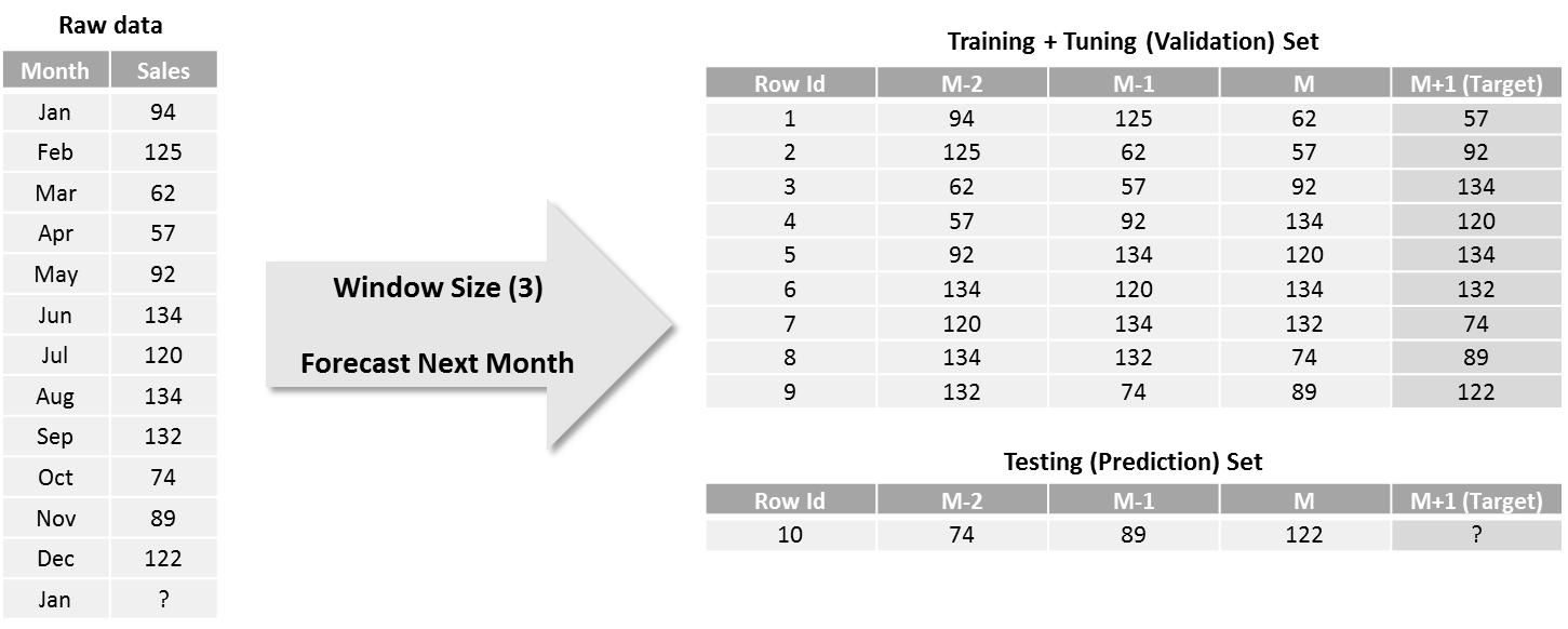
One-step-ahead forecasting is an easy-to-implement case wherein the model is trained on the next time period using N (window size) previous observations.

However, for multi-step forecasting, as more than one value needs to be forecasted, there are several approaches for model creation and prediction. Now, let’s take the same 12 monthly observations as above, but forecast sales of next 3 months instead of 1.

Let’s have a look at various approaches of model creation and prediction one-by-one.

Recursive Strategy:

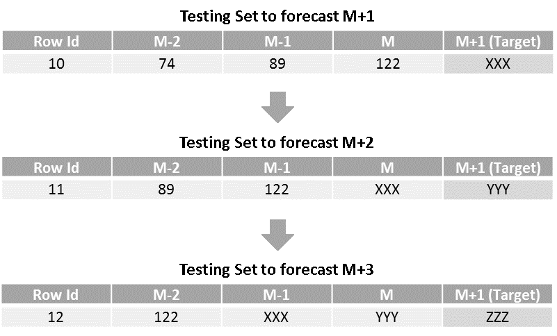
• Here, the idea is to train the model to forecast for the next time period and use it iteratively to generate forecasts for all the future time periods. So, the training set and model for this approach remains the same as that of the one-step forecasting approach. And, we use the testing set to generate next month (M+1) forecast. Once we have M+1 forecast, we slide the window by one time-period (shift observations by one month in this case) to create the next row of testing sets, which holds the latest forecasted value under column M as shown below. Then, we use this row as a testing set and generate M+2 forecast using the same model. Similarly, all the subsequent forecasts are generated by repeating these steps.

As forecasts generated in the prior steps are used for the prediction of next forecasts iteratively, it is termed as a recursive strategy. The advantage of this approach is that only one model is created and hence memory and computation requirements are relatively low. For the same reason, this approach is widely used for multi-step forecasting when the forecasting horizon is medium to long-term. On the other hand, as the forecasted values are used for the subsequent predictions, the model has a tendency to accumulate errors and therefore forecasting accuracy may drop significantly as forecasting horizon increases. Also, time taken for prediction is higher for the distant forecasts as it needs to wait for all prior forecasts to be generated.

Direct Strategy:

• As opposed to the recursive strategy, here, we’ll create 3 different models, one each for next month, M+2 and M+3 forecasts. The training and testing datasets would look as below.

As we can see, the target observation in training set for M+2 and M+3 models are 2 and 3 time periods ahead of the M or the latest value. Also, the number of training rows keeps on reducing for models that are farther in the time period. Prediction or testing sets for all 3 models are same with each giving forecast for different months.

The benefit of this approach is that it is easy-to-implement and errors does not accumulate like in case of recursive strategy. Additionally, the time taken for prediction is relatively low as all models can run independently to predict multi-step forecasts. But, on the other hand, this approach is an overkill when number of forecasts to be made increases beyond 10-15 as you need to have that many models deployed for prediction. With more number of models, you need to account for extra computation and memory requirements. Also, as the models are independent of each other, there is no scope for modeling the statistical dependencies among the predictions.

Hybrid or DirRec Strategy:

This strategy makes use of the philosophies of both recursive and direct strategies. Similar to direct strategy, separate models are created for each time-period in the forecasting horizon with the difference being that the size of the sliding window keeps on increasing for each step. And similar to the recursive strategy, the forecast generated in step one is fed to the second model to generate the forecast for step two and so on. So, the resulting training and testing dataset would look as shown below.

• Although the hybrid strategy improves the forecasting accuracy by combining the advantages of both recursive and direct strategies, it is relatively complex and has high computational and memory requirements. Therefore, it is advisable to avoid this strategy for use cases where the dollar impact of units increase in accuracy over recursive/direct is relatively low.

Multiple Output Strategies:

• There are more advanced strategies which work on multiple input multiple output concept unlike these 3 which are based on multiple input single output structure. They are MIMO (multiple input multiple output) and DIRMO (Direct + MIMO) strategies, but it requires special algorithms like LSTM that are capable of predicting multiple outputs. However, computation time and memory required to train these models is very high. Therefore, we have not discussed these strategies in detail in this article.

These are some of the approaches to forecasting multi-step time-series as supervised ML problem. There are pros and cons of each strategy in terms of forecasting errors, number of models to be built, computation time, memory requirement, complexity of implementation, assumption of inter-dependence among forecasts. The selection of right strategy is made considering these trade-offs in mind.

Model Granularity Selection:

So far, we have discussed how a supervised ML model can be created and used to make forecasts from a single time-series. However, in reality, a majority of use cases require forecasting over few tens to few thousands of time-series’ like weather forecasting across different weather stations, demand forecasting for various products in a company’s catalog, cash balance forecasting for different accounts in the bank etc. And there exist groups of time-series’ that are similar to a few others and different from the remaining ones in terms of observed trend, seasonality, cyclic components.

As creating separate models for these many time-series’ may not be a feasible solution for production deployment perspective, it is advisable that we combine them into few clusters containing series’ that are similar within a group and different across groups so that one ML model can be created for each cluster. As shown below, the selection of modeling granularity is a decision that needs to consider trade-offs among cost, complexity, accuracy, scalability and hence we suggest to go with a balanced approach that uses at least one level of clustering.

Figure 1 Granularity selection for product sales forecasting

For clustering, we can use company’s internal product hierarchy (assuming products within a category have similar demand) or a statistical clustering algorithm suitable for time-series data or a rule-based clustering based on the range of values or domain-specific knowledge.

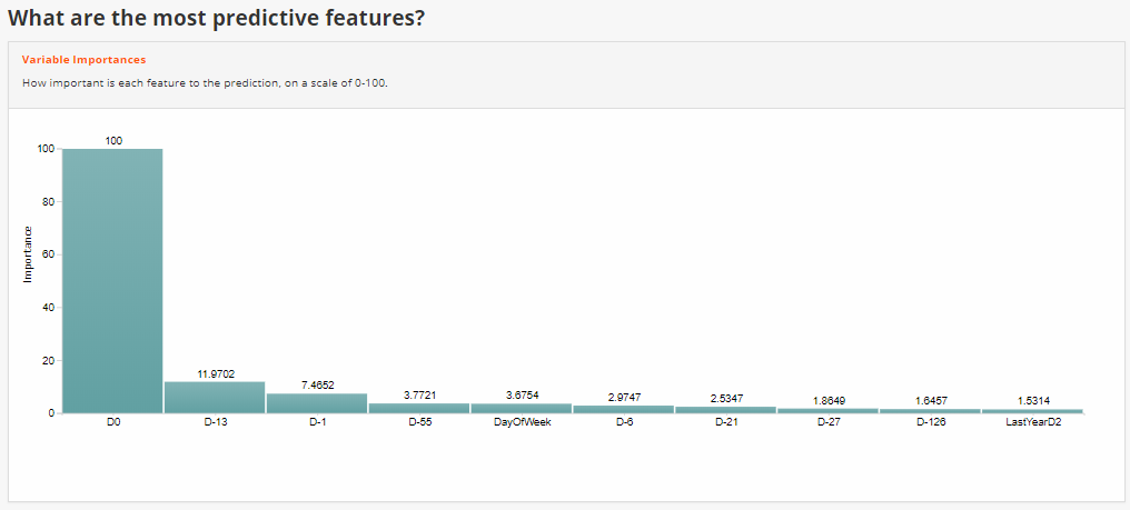
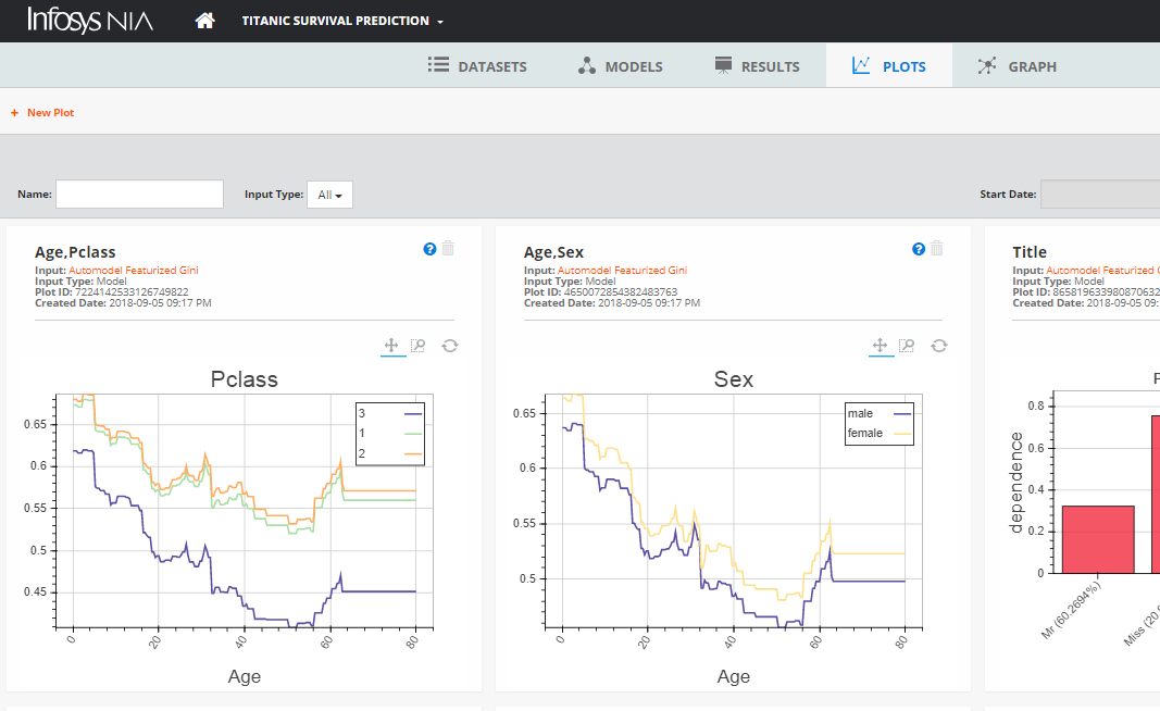
Throughout this journey, we have used the Infosys NIA Advanced ML Platform, which is an end-to-end data science platform that provides tools and frameworks to automate these ML tasks.

Figure 2, 3 Model interpretability features like most important predictors and Partial Dependence Plots from Infosys NIA

Conclusion

With the increased prominence of ML in last decade, we have seen a steady increase in the number of use cases and data science competitions where supervised learning algorithms like tree-based or Deep Learning-based have outperformed statistical algorithms like ARIMA, ETS, etc. These are some of the learnings that we acquired while solving the time-series forecasting using ML methods for use cases like bank account balance forecasting and product sales forecasting. We hope that these learnings help readers solve time-series problems using ML methods efficiently.