Building a Product Recommendation Engine With Neo4j — No ML Library Required

When many developers think about recommendation engines, they think of machine learning: collaborative filtering models, matrix factorization, embedding vectors, and training pipelines. What surprises many people is that you can build a genuinely useful recommendation system with nothing more than a graph database and several Cypher queries. No scikit-learn, no TensorFlow, no model training. Just the natural structure of the data doing the work.

In this article, we'll build a product recommendation engine on top of Neo4j Aura using two Jupyter notebooks. The first generates a realistic synthetic dataset and loads it into Aura. The second runs four recommendation queries directly in Cypher and visualizes the results with Plotly. Everything runs locally in a Python virtual environment against a free cloud Neo4j instance.

The full source code is available on GitHub.

Why Graphs Are a Natural Fit for Recommendations

The core intuition behind most recommendation approaches is relationship: this customer bought that product, those products appear together in the same order, this product shares attributes with that one. In a relational database, capturing these relationships means multiple self-joins across large tables. A query like "find products bought by customers who also bought what this customer bought" quickly becomes difficult to write and expensive to execute at scale.

In a graph, that same question is a traversal. We follow edges from a customer to the products they purchased, hop across to other customers who share those products, and collect what else those customers bought. The query is short, the intent is clear, and the graph engine is optimized for exactly this kind of path-following work.

Prerequisites

AuraDB is Neo4j's fully managed cloud database. A free tier is available with no credit card required.

• Sign up at Get Started for Free.
• Create a new AuraDB Free instance.
• When the instance is created, download or note the credentials — the connection URI, username, and password.
• Once the instance is running, open the Query tab and connect to the instance.
• Confirm it's empty with MATCH (n) RETURN count(n) which should return 0

A virtual environment is highly recommended. For example:

python3 -m venv ~/recommendation-engine-env
source ~/recommendation-engine-env/bin/activate

Before starting Jupyter, export the connection details as environment variables in your shell:

export NEO4J_URI="neo4j+s://xxxx.databases.neo4j.io"
export NEO4J_USERNAME="your_username_here"
export NEO4J_PASSWORD="your_password_here"

The Graph Model

Before we write any code, let's define the graph. We have four node types and three relationship types.

Nodes

• Customer – id, name, email, city, country.
• Product – id, name, description, price.
• Category – name (e.g., Electronics, Clothing, Books).
• Tag – name (e.g. "wireless", "eco-friendly", "premium").

Relationships

• (:Customer)-[:PURCHASED {order_id, quantity, order_date}]->(:Product) — order metadata lives on the relationship rather than a separate Order node, which keeps our Cypher clean.
• (:Product)-[:BELONGS_TO]->(:Category)
• (:Product)-[:TAGGED_WITH]->(:Tag)

The decision to put order_id, quantity and order_date on the PURCHASED relationship is worth discussing. It means a single customer can have multiple PURCHASED relationships to the same product (each with a different order_id) and we can group by order_id to find products that appeared together in the same basket — which is exactly what our co-purchase query needs. Figure 1 illustrates exactly this point, as we have a customer, two products, and the same order_id.

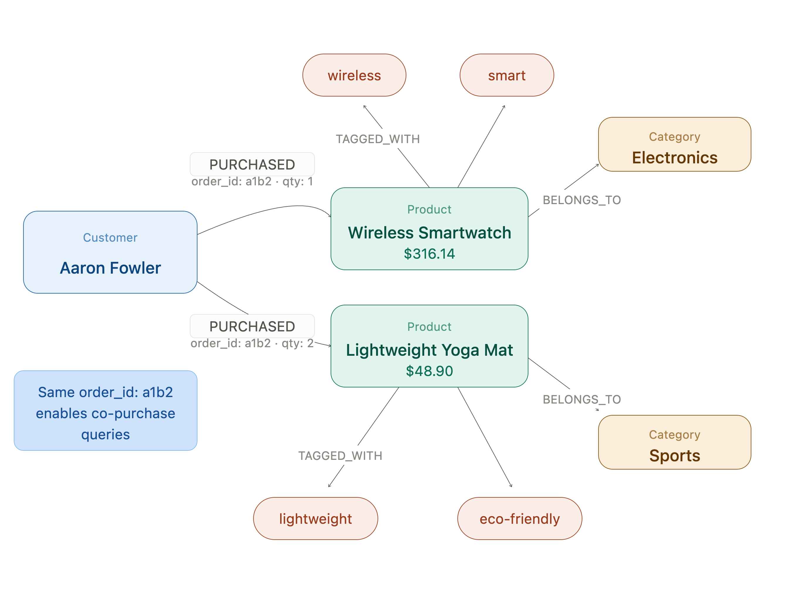
Figure 1. Shared order_id enables co-purchase queries

Notebook 1: Data Generation and Loading

Rather than sourcing an external dataset, we'll generate synthetic data using Faker. This keeps the notebook fully self-contained, and readers can run it as-is without downloading anything.

We'll generate 2,000 customers, 500 products across 15 categories, and 20,000 orders. Each order is a basket of several products sharing the same order_id — this is the key design decision that makes the frequently-bought-together query work. With an average basket of 3 products, we end up with around 60,000 PURCHASED relationships in the graph.

Realistic Product Names

Faker's default catch_phrase() method produces output like "Proactive exuding encoding" — readable enough for a demo but not really useful in an article. Instead, we define a PRODUCT_VOCAB dictionary keyed by category, each containing lists of adjectives, nouns, use cases, and benefit statements. A product name is then a simple combination, as follows:

def make_product_name(category):
    vocab = PRODUCT_VOCAB[category]
    adj  = random.choice(vocab["adjectives"])
    noun = random.choice(vocab["nouns"])
    return f"{adj} {noun}"

def make_product_description(category, name):
    vocab    = PRODUCT_VOCAB[category]
    use_case = random.choice(vocab["use_cases"])
    benefit  = random.choice(vocab["benefits"])
    return f"The {name} is designed for {use_case}. {benefit}."

This gives us names like "Wireless Noise-Canceling Earbuds," "Organic Ground Coffee" and "Ergonomic Lumbar Support Cushion" — realistic enough to make the recommendation output meaningful.

Basket-Based Order Generation

Each order picks a random customer, generates a unique order_id, and samples several products into a basket. We then flatten the basket into individual order lines, each carrying the shared order_id:

orders = []
for _ in range(NUM_ORDERS):
    order_id   = str(uuid.uuid4())
    customer   = random.choice(customers)
    order_date = (start_date + timedelta(days=random.randint(0, 730))).strftime("%Y-%m-%d")
    basket     = random.sample(products, k=random.randint(2, 4))
    for product in basket:
        orders.append({
            "order_id":    order_id,
            "customer_id": customer["id"],
            "product_id":  product["id"],
            "quantity":    random.randint(1, 5),
            "order_date":  order_date
        })

Loading Into Aura

Data loading is in batches of 100 using MERGE statements. To show progress during the load, we'll use tqdm as ~60,000 order lines can take several minutes, and the progress bars make it easy to see what's happening:

with driver.session() as session:

    customer_batches = range(0, len(customers), BATCH_SIZE)
    for i in tqdm(customer_batches, desc="Loading customers", unit="batch", colour="#1f77b4"):
        session.execute_write(load_customers, customers[i:i+BATCH_SIZE])

    product_batches = range(0, len(products), BATCH_SIZE)
    for i in tqdm(product_batches, desc="Loading products ", unit="batch", colour="#1f77b4"):
        session.execute_write(load_products, products[i:i+BATCH_SIZE])

    for product_id, tags in tqdm(product_tags.items(), desc="Loading tags     ", unit="product", colour="#1f77b4"):
        session.execute_write(load_tags, product_id, tags)

    order_batches = range(0, len(orders), BATCH_SIZE)
    for i in tqdm(order_batches, desc="Loading orders   ", unit="batch", colour="#1f77b4"):
        session.execute_write(load_orders, orders[i:i+BATCH_SIZE])

A verification query at the end confirms the counts.

The Four Recommendation Queries

Notebook 2 runs four Cypher queries against the loaded graph, each implementing a different recommendation strategy. Before running any query, we fetch a stable seed customer, product, and category:

with driver.session() as session:

    customer = session.run("""
        MATCH (c:Customer)
        RETURN c.id AS customer_id, c.name AS customer_name
        ORDER BY c.name ASC
        LIMIT 1
    """).single()

    product = session.run("""
        MATCH (p:Product)<-[r:PURCHASED]-()
        RETURN p.id AS product_id, p.name AS product_name, count(r) AS order_count
        ORDER BY order_count DESC
        LIMIT 1
    """).single()

    top_cat = session.run("""
        MATCH (p:Product)-[:BELONGS_TO]->(cat:Category)
        RETURN cat.name AS category, count(p) AS total
        ORDER BY total DESC
        LIMIT 1
    """).single()

We pick the alphabetically first customer for consistency, the most-purchased product to ensure co-purchase data exists, and the category with the most products for the trending query. This makes the notebook reproducible across runs.

Query 1: Collaborative Filtering

The classic "customers who bought this also bought" approach. We find customers who share at least one purchased product with the seed customer, then collect what else those customers bought — excluding anything the seed customer already purchased.

def collaborative_filtering(tx, customer_id, limit=5):
    result = tx.run("""
        MATCH (target:Customer {id: $customer_id})-[:PURCHASED]->(p:Product)
              <-[:PURCHASED]-(other:Customer)-[:PURCHASED]->(rec:Product)
        WHERE NOT (target)-[:PURCHASED]->(rec)
        RETURN rec.id       AS id,
               rec.name     AS product,
               rec.price    AS price,
               count(other) AS score
        ORDER BY score DESC, id ASC
        LIMIT $limit
    """, customer_id=customer_id, limit=limit)
    return result.data()

The score is the number of other customers whose purchasing overlap with our target customer also led them to buy the recommended product. A higher score means more customers in the overlap group bought it, making it a stronger signal. In Cypher, the traversal reads almost like the description: start at the target customer, follow PURCHASED edges to products, hop to other customers who bought the same products, then follow their PURCHASED edges to new products.

Query 2: Frequently Bought Together

This query finds products that appeared in the same order as the seed product. The key is matching on order_id across two PURCHASED relationships from the same customer:

def frequently_bought_together(tx, product_id, limit=5):
    result = tx.run("""
        MATCH (p:Product {id: $product_id})<-[r1:PURCHASED]-(c:Customer)
              -[r2:PURCHASED]->(other:Product)
        WHERE r1.order_id = r2.order_id
          AND other.id <> $product_id
        RETURN other.id    AS id,
               other.name  AS product,
               other.price AS price,
               count(c)    AS frequency
        ORDER BY frequency DESC, id ASC
        LIMIT $limit
    """, product_id=product_id, limit=limit)
    return result.data()

The WHERE r1.order_id = r2.order_id clause is what makes this work. It constrains the traversal to only consider cases where both products were part of the same order, not just bought by the same customer at different times. frequency counts how many distinct customers placed an order containing both products together.

Query 3: Content-Based Filtering

Rather than looking at purchase behavior, this query finds products similar to the seed product based on shared tags. The more tags two products have in common, the more similar they are:

def content_based(tx, product_id, limit=5):
    result = tx.run("""
        MATCH (p:Product {id: $product_id})-[:TAGGED_WITH]->(t:Tag)
              <-[:TAGGED_WITH]-(rec:Product)
        WHERE rec.id <> $product_id
        RETURN rec.id       AS id,
               rec.name     AS product,
               rec.price    AS price,
               count(t)     AS shared_tags
        ORDER BY shared_tags DESC, id ASC
        LIMIT $limit
    """, product_id=product_id, limit=limit)
    return result.data()

The traversal goes outward from the seed product through its tags, then back inward to any other product that shares those same tags. count(t) gives the number of shared tags, which serves as a simple but effective similarity score. This approach works without any purchase history, making it useful for recommending products to new customers or for newly listed products with no order data yet.

Query 4: Trending in Category

This query finds the most purchased products in the top category within a fixed date window. In our case, this is from 2024-10-01 onwards:

def trending_in_category(tx, category_name, cutoff="2024-10-01", limit=5):
    result = tx.run("""
        MATCH (p:Product)-[:BELONGS_TO]->(cat:Category {name: $category_name})
        MATCH (:Customer)-[r:PURCHASED]->(p)
        WHERE date(r.order_date) >= date($cutoff)
        RETURN p.id     AS id,
               p.name   AS product,
               p.price  AS price,
               count(r) AS purchases
        ORDER BY purchases DESC, id ASC
        LIMIT $limit
    """, category_name=category_name, cutoff=cutoff, limit=limit)
    return result.data()

We use date() conversion on the stored string order_date to enable date comparison. count(r) counts individual PURCHASED relationships rather than distinct customers, so a customer who bought the same product multiple times within the window is counted each time — reflecting genuine demand volume rather than unique buyer count.

Notebook 2: Results

Each query outputs a table followed by a Plotly horizontal bar chart. Here are the results for our seed data.

Collaborative Filtering

Figure 2 returns five products. The top recommendation is An Introduction to Public Speaking, driven by the number of customers whose purchasing overlap with Aaron Boyd also led them to buy it. Heavy-Duty Cable Management Box and Educational Coding Robot follow closely, showing that the overlap group bought broadly across categories rather than clustering in one area.

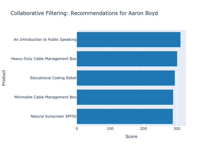
Figure 2. Collaborative filtering

Frequently Bought Together

Figure 3 shows products co-purchased with the Durable Grooming Brush in the same order basket. The top results — Waterproof Hammock and Natural Body Lotion at frequency 4, followed by Adjustable Lumbar Support Cushion, Sugar-Free Collagen Powder and Slim-Fit Hiking Vest at frequency 3 — show which products most commonly appeared alongside the seed product in the same order. The cross-category spread here (Beauty, Outdoor, Clothing, Health, Office) is a feature of random synthetic data; in a real system, we'd expect more category clustering.

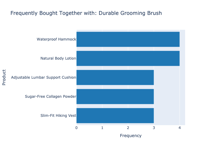
Figure 3. Frequently bought together

Content-Based Filtering

Figure 4 finds products sharing the most tags with the seed product. All five results share 2 tags with the Durable Grooming Brush — Smart Mechanical Keyboard, Waterproof Toiletry Bag, Ergonomic Whiteboard, Cold-Pressed Hot Sauce, and Durable Dumbbell Pair. The cross-category reach (Sports, Food & Drink, Office, Travel, Electronics) illustrates the tag graph doing its job: shared attributes like "durable" or "waterproof" create similarity links that cross category boundaries, which is useful for surface-level discovery recommendations.

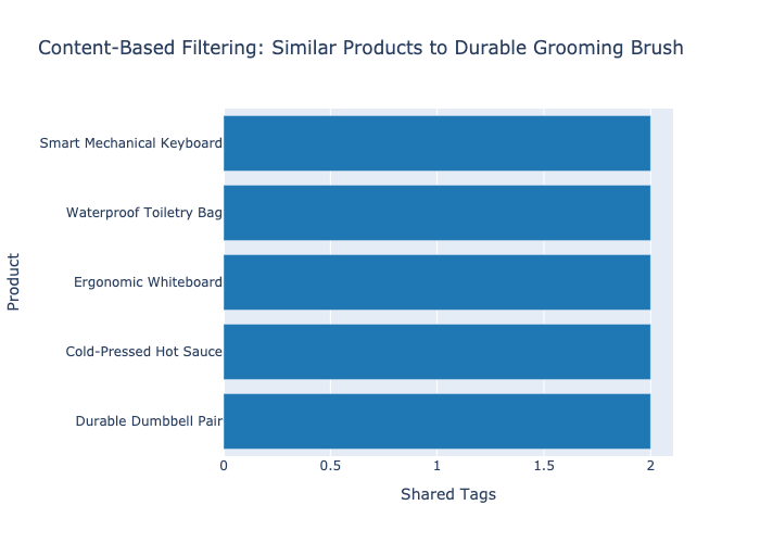
Figure 4. Content-based filtering

Trending in Category

Figure 5 shows the top 5 products in Toys — the category with the most products in our graph — with purchase counts from 2024-10-01 onwards. Battery-Free Coding Robot leads, followed by Battery-Free Building Blocks Set, Interactive Remote Control Car, Wooden Magnetic Drawing Board, and Creative Puzzle Game. The scores are tight here, which makes sense because within a single category over a fixed time window, popular products tend to cluster around similar purchase volumes.

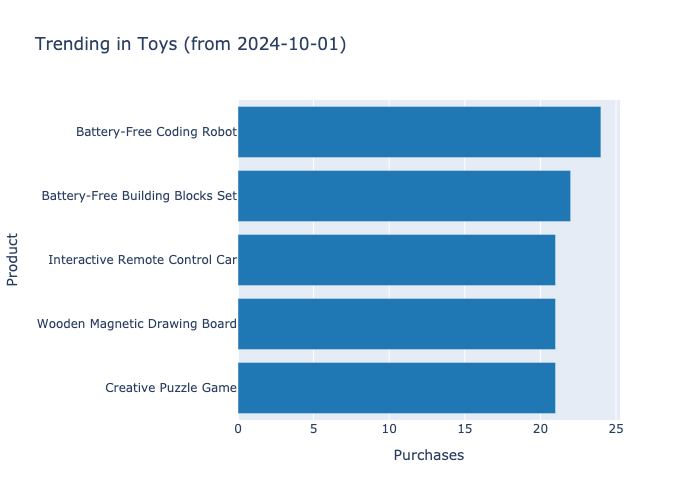
Figure 5. Trending

Summary

We've built a working product recommendation engine using nothing but Neo4j, Cypher, and a few Python libraries. No ML framework, no training data, no model deployment. The four queries cover the most common recommendation patterns in production systems:

• Collaborative filtering
• Co-purchase analysis
• Content similarity
• Trending detection

The graph model is the foundation that makes this possible. Storing orders as relationships with properties means co-purchase queries are a natural traversal rather than a complex join. Adding tags as nodes means similarity queries are just path-matching. Because everything lives in the same graph, we can also combine these approaches. For example, filtering collaborative filtering results by tag similarity using a single extended Cypher query.

The full source code is available on GitHub.