From 30s to 200ms: Optimizing Multidimensional Time Series Analysis at Scale

Monitoring production systems in real-time is crucial for reliability. Multidimensional anomaly detection is a very helpful tool in this regard. However, it does require time-series analysis to be blazing fast. This follow-up blog shows how to speed them up by using different strategies like indexing, filtering, bucketing, etc., to achieve a consistent performance in the 100s of ms range.

Recap

Most teams learn the hard way that global all-green dashboards can hide real incidents in a single cohort. In Part 1: A Guide to Multidimensional Anomaly Detection, we covered the why and the solution blueprint. 

This highly requested follow‑up focuses on the narrower problem of data-engine efficiency: How do you make time‑series queries blazing-fast and cost-effective to enable automated systems to discover and triage errors in production on live data? This becomes more prominent as the data volume increases, combined with finer time granularities and higher dimensionality.

A couple of key terminologies:

• Metric: aggregate over events (e.g.,COUNT(*),SUM(revenue), p95(latency_ms)
• Dimensions: columns you filter/group on (e.g., country, device, app_version)

Problem Space

Anatomy of a SQL Query

Here is the SQL structure for the most common time-series anomaly-detection dataframes.

-- Build a time vs aggregated metric dataframe for a given window and given dimensions
SELECT 
	TIME_BUCKET_FN('${timeColumn}', '${timeColumnFormat}', '${monitoringGranularity}') AS timeBucket, 
    AGG_FN(metricColumn) as metric
FROM metric_data
WHERE timeBucket in <time range>
	AND country = 'US' AND <other dimensions>
GROUP BY timeBucket

Most anomaly detection algorithms follow the above standard schema that entails the following:

• Time bucket: This is the aggregation unit. Bucket size ranges from short durations of a min to longer durations like an hour, a day, and sometimes even a week or a month
• Aggregated metric: This is the aggregated value of the metric during the time bucket
• Dimension value(s): Overall value or the value of a particular dimension, could be a list of them for multidimensional alerts.

Latency and Throughput Performance

Query performance is crucial so that downstream alerting systems can consume the data fast enough to ensure that the system is reliable. Imagine running 1 min/5 min level alerting on a 200+ TB dataset across 10 metrics for 500 dimensions. This is not a hypothetical scenario but something that we solved in production for DoorDash (see here). We saw this pattern repeat across different use cases.

Here are the key challenges

• Time column grouping: This appears trivial, but it's not. Grouping different timestamps into 1m/5m/15m/1h granularities can get really expensive as the dataset scales
• Aggregation: We need the aggregated value of the metric across different GROUP BY queries to be performant. This can get trickier for expensive aggregations like COUNT DISTINCT.
• Throughput: For multidimensional alerts going into a 1000s of dimensions, we need these queries to be highly memory efficient so that we can serve these 1k QPS query bursts at scale without choking the system.

Approach

The approach here is to measure each bottleneck and optimize 1 by 1. Let's start with the timestamp grouping issue.

Inverted Index for Popular Dimensions

When querying time-series slices across different dimensions, it often helps to have inverted indexes in place to make it easy to filter by WHERE. Of course, the more complex piece here is the metric value of this dimension slice, and that is handled by having a startree index or equivalent.

This simple strategy to deploy an inverted index works really well for a variety of use cases.

Approximate Results

Some aggregation functions are more expensive than others. Count Distinct, for example, can be very expensive since it requires a complete shuffle of keys to accurately report the number of distinct ones. Instead of exact results, there are efficient alternatives like DISTINCTCOUNTHLL or the more recent DISTINCTCOUNTULL function which can report a reasonable approximate but can be much faster to compute. 

Time Column Performance

The timestamp is usually stored as epoch long. Scanning millions of rows and performing a mod or division operation on every single timestamp at runtime kills the CPU. Pre-calculating this turns a calculation task into a simple fetch. However, sometimes it is stored as string and other complex formats that can greatly affect query performance if not natively supported by the engine.

Also, converting the long timestamp into an appropriate time bucket can itself be a very expensive operation, especially if you have a large dataset with fine-granularity datapoints on epoch millis. Converting these epochs to the nearest minute/5m (for say 1m/5m monitoring) could mean running a transform function and then performing GROUP BY on the transformed value of the time column, which can be quite slow at runtime. A simple strategy to speed up these queries is by creating derived columns, like say timestamp_1m, timestamp_5m during ingestion time that trades runtime performance for disk storage. This is often a common tradeoff.

Sometimes databases extend first-class support to this kind of bucketing. For example, in Apache Pinot, you have a timestamp Index that automatically creates materialized columns for configured granularities.

{
  "fieldConfigList": [
    {
      "name": "event_time",
      "encodingType": "DICTIONARY",
      "indexTypes": ["TIMESTAMP"],
      "timestampConfig": {
        "granularities": [
          "MINUTE",   // 1-minute bucket
          "HOUR",     // hourly bucket
          "DAY"       // daily bucket
        ]
      }
    }
  ]
}

Disclosure: I work at Startree Inc on Apache Pinot and Startree ThirdEye, which is why I’m using it here as an example implementation. The concepts directly extend to other stacks, too.

With this style of configuration, Pinot exposes materialized columns like:

• $event_time$MINUTE 
• $event_time$HOUR 
• $event_time$DAY

Thus, during query execution, Pinot is able to use these materialized values directly instead of computing the time buckets repeatedly on every query, saving a lot of compute.

Metric Aggregation Performance

Metric is the actual value of the time series. This can be simple aggregations like sum(views) or avg(revenue) or can be more interesting like p99(latency). For large datasets, this can also lead to a performance bottleneck. One of the ways of speeding up the query is to use precomputation. Caching the overall metric is often easy. However, caching different slices of the data can be expensive. So the 2 ends of the spectrum look like this. On one end, you always compute on the fly. On the other hand, you precompute everything effectively by building a CUBE. However, neither of these extremes works in practice.

Usually, the workable approach here is to trade off time and space by partially aggregating the dimensions that serve the business use case and ignoring the rest. One of the ways Apache Pinot handles this is via the Startree Index. By using such a construct, Pinot can cache some of the aggregated values ahead of time, dramatically reducing query latency. A hypothetical example is shared below.

{
  "tableIndexConfig": {
    "loadMode": "MMAP",
    "starTreeIndexConfigs": [
      {
        "dimensionColumns": [
          "country",
          "deviceType",
          "$event_time$HOUR"
        ],
        "metricAggregations": [
          {
            "column": "views",
            "function": "SUM"
          }
        ],
        "maxLeafRecords": 10000,
        "skipStarNodeCreationForDimensions": []
      }
    ]
  }
}

Results

Here are the results for the above strategy when applied to a production use case for DoorDash. You can read the full story here. 

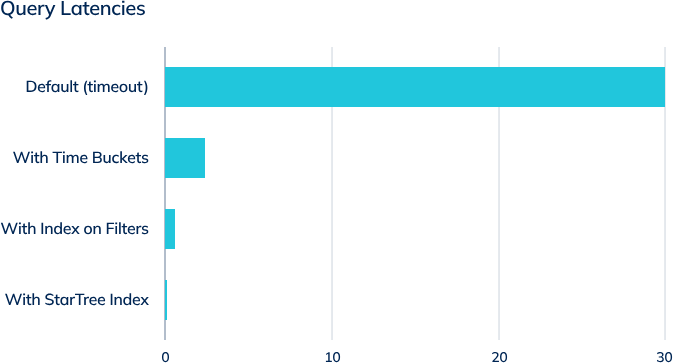
By combining these strategies, one can significantly improve the query performance. In the Default (no optimization) case above, the queries were actually timing out. But by systematically attacking each bottleneck using the above strategies, we were able to bring the average query performance well under sub-second latencies.

Wrap Up

Query optimization at scale can be a challenging problem. However, if we approach the problem from first principles and start from the use case to the data modeling to actual performance, the problem breaks down and becomes a lot more tangible. In this article, we walked through different strategies that we use in production to build reliable and performant alerting at scale. Using this approach, we were able to reduce the query latency from 30s (timeout) to under 200ms.

I hope this was helpful, and I'd love to hear and learn from your experiences.

Disclosure: I work at Startree Inc on Apache Pinot and Startree ThirdEye.