Essential Techniques for Production Vector Search Systems, Part 5: Reranking
Proven techniques for production vector search, including when to use each one, how to combine them effectively, and trade-offs to understand before deployment.
Join the DZone community and get the full member experience.
Join For FreeAfter implementing vector search systems at multiple companies, I wanted to document efficient techniques that can be very helpful for successful production deployments.
I want to present these techniques by showcasing when to apply each one, how they complement each other, and the trade-offs they introduce. This will be a multi-part series that introduces all of the techniques one by one in each article. I have also included code snippets to quickly test each technique.
Before we get into the real details, let us look at the prerequisites and setup.
For ease of understanding and use, I am using the free cloud tier from Qdrant for all of the demonstrations below.
Steps to Set Up Qdrant Cloud
Step 1: Get a Free Qdrant Cloud Cluster
- Sign up at https://cloud.qdrant.io.
- Create a free cluster
- Click "Create Cluster."
- Select Free Tier.
- Choose a region closest to you.
- Wait for the cluster to be provisioned.
- Capture your credentials.
- Cluster URL: https://xxxxxxxx-xxxx-xxxx-xxxx-xxxxxxxxxxxx.us-east.aws.cloud.qdrant.io:6333.
- API Key: Click "API Keys" → "Generate" → Copy the key.
Step 2: Install Python Dependencies
pip install qdrant-client fastembed numpyRecommended versions:
- qdrant-client >= 1.7.0
- fastembed >= 0.2.0
- numpy >= 1.24.0
- python-dotenv >= 1.0.0
Step 3: Set Environment Variables or Create a .env File
# Add to your ~/.bashrc or ~/.zshrc
export QDRANT_URL="https://your-cluster-url.cloud.qdrant.io:6333"
export QDRANT_API_KEY="your-api-key-here"
Create a .env file in the project directory with the following content. Remember to add .env to your .gitignore to avoid committing credentials.
# .env file
QDRANT_URL=https://your-cluster-url.cloud.qdrant.io:6333
QDRANT_API_KEY=your-api-key-here
Step 4: Verify Connection
We can verify the connection to the Qdrant collection with the following script. From this point onward, I am assuming the .env setup is complete.
from qdrant_client import QdrantClient
from dotenv import load_dotenv
import os

# Load environment variables from .env file
load_dotenv()

# Initialize client
client = QdrantClient(
    url=os.getenv("QDRANT_URL"),
    api_key=os.getenv("QDRANT_API_KEY"),
)

# Test connection
try:
    collections = client.get_collections()
    print(f" Connected successfully!")
    print(f"   Current collections: {len(collections.collections)}")
except Exception as e:
    print(f" Connection failed: {e}")
    print("   Check your .env file has QDRANT_URL and QDRANT_API_KEY")
Expected Output:
python verify-connection.py
Connected successfully!
Current collections: 2
Now that we have the setup out of the way, we can get into the meat of the article.
Before the deep dive into reranking, let us look at a high-level overview of the techniques we have covered so far, and also the last one we are covering in this part.
| Technique | problems solved | performance impact | complexity |
|---|---|---|---|
| Hybrid Search | We will miss exact matches if we employ semantic search purely. | Huge increase in the accuracy, closer to 16% | Medium |
| Binary Quantization | Memory costs scale linearly with data. | 40X memory reduction, 15% faster | Low |
| Filterable HNSW | Not a good practice to apply post-filtering as it wastes computation. | 5X faster filtered queries | Medium |
| Multi Vector Search | A single embedding will not be able to capture the importance of various fields. | Handles queries from multiple fields, such as title vs description, and requires two times more storage. | Medium |
| Reranking | Optimized vector search for speed over precision. | Deeper semantic understanding, 15-20% ranking improvement | High |
Keep in mind that production systems typically combine two to four of these techniques.
For example, a typical e-commerce website might use hybrid search, binary quantization, and filterable HNSW.
We covered Hybrid Search in the first part of the series, Binary Quantization in the second part, filterable HNSW in the third part, and multi-vector search in the 4th part. In the final part, we will cover reranking.
Reranking
All the techniques we have covered so far have focused on quickly identifying the right candidates. Reranking is about ensuring the right result shows up as the number one choice. These are two different spectrums of search. Since we have looked at the first aspect in all four parts so far, let us now look at the retrieval quality aspect in this article.
The core concept of reranking allows the system to read both the query and the document together at query time, attending to every token in both. It might not scale to the corpus, but it is very efficient at providing a deeper understanding for a shortlist of 20-100 candidates.
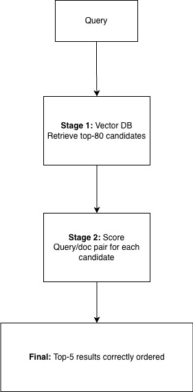
Let us look at the pattern we follow for retrieval in the case of reranking.
Stage 1: Retrieve as many candidates as possible quickly. This is primarily what we have seen in the first 4 parts of this series.
Stage 2: Rescore the shortlist with the full query document attention and return the true top-k, even if that means adding latency.
High-Level Conceptual Flow Diagram for Reranking
Let us now look at the two-step process with the help of the following conceptual flow diagram
Let us now take a look at it in more detail with the code below.
"""
Example: two-stage retrieval with cross-encoder reranking.

Stage 1 — Bi-encoder (vector): retrieve many candidates quickly (~tens of ms).
Stage 2 — Cross-encoder: rescore (query, document) pairs and take top 5 (~hundreds of ms).

This demo uses title-only Stage 1 when the collection has a `title` vector: that mimics a
common production pattern (cheap first pass on short fields) and often misorders results
vs the full product text — so reranking’s lift is visible (correct part moves to #1).
"""

from dotenv import load_dotenv

from multi_vector import (
    create_demo_collection,
    get_collection_vector_names,
    get_qdrant_client,
)
from rerank_search import (
    display_two_stage_result,
    get_cross_encoder,
    two_stage_retrieve,
    warm_bi_encoder,
)

load_dotenv()

client = get_qdrant_client()
EXISTING_COLLECTION_NAME = "automotive_parts"
DEMO_COLLECTION_NAME = "multi_vector_demo"

STAGE1_LIMIT = 80
STAGE2_TOP_K = 5
TYPICAL_S1_MS = 45.0
TYPICAL_S2_MS = 190.0

# --- Collection setup (same pattern as multi_vector_example.py) ---
print("=" * 80)
print("RERANKING DEMO — Collection setup")
print("=" * 80)

available_vectors = get_collection_vector_names(EXISTING_COLLECTION_NAME, client)

if available_vectors:
    print(f"Using '{EXISTING_COLLECTION_NAME}' with vectors: {available_vectors}")
    COLLECTION_NAME = EXISTING_COLLECTION_NAME
    vector_names = available_vectors[:2]
    if len(vector_names) == 1:
        vector_names = [vector_names[0], vector_names[0]]
    weights = {name: 1.0 / len(vector_names) for name in vector_names}
else:
    print(f"No named vectors in '{EXISTING_COLLECTION_NAME}'. Using demo collection.")
    if not create_demo_collection(DEMO_COLLECTION_NAME, client, force_recreate=False):
        print("Failed to create or open demo collection. Exiting.")
        exit(1)
    COLLECTION_NAME = DEMO_COLLECTION_NAME
    vector_names = ["title", "description"]
    weights = {"title": 0.6, "description": 0.4}

# Title-only Stage 1 when possible — makes rerank “rescue” visible on small catalogs
if "title" in vector_names:
    STAGE1_MODE = "title"
    STAGE1_VECTOR = "title"
else:
    STAGE1_MODE = "multi"
    STAGE1_VECTOR = None

print(f"Collection: {COLLECTION_NAME}")
print(f"Stage 1: up to {STAGE1_LIMIT} candidates using {STAGE1_MODE} (lean / fast first pass).")
print(f"Stage 2: cross-encoder rerank → top {STAGE2_TOP_K} (full title + description text).")
if STAGE1_MODE == "title":
    print(
        "Note: Title-only Stage 1 ignores description — e.g. 'Wheel Speed Sensor' loses\n"
        "      explicit ABS context; generic 'Brake … Sensor' titles win until rerank.\n"
    )
print()

# Warm models (first run downloads cross-encoder weights)
print("Loading bi-encoder and cross-encoder (first run may download models)...")
warm_bi_encoder()
ce = get_cross_encoder()
print("Cross-encoder ready (cross-encoder/ms-marco-MiniLM-L-6-v2).")
print()

# --- Scenario 1: ABS-specific intent ---
print("=" * 80)
print('SCENARIO 1: Complex query — "brake sensor for ABS system"')
print("=" * 80)
print(
    "Title-only retrieval matches literal 'brake' + 'sensor' in titles; the true ABS part\n"
    "is titled 'Wheel Speed Sensor' (ABS only in description). Reranking reads full text.\n"
)

target_abs = "ABS Wheel Speed Sensor"
r1 = two_stage_retrieve(
    COLLECTION_NAME,
    "brake sensor for ABS system",
    vector_names,
    weights,
    client,
    stage1_limit=STAGE1_LIMIT,
    stage2_top_k=STAGE2_TOP_K,
    cross_encoder=ce,
    stage1_mode=STAGE1_MODE,
    stage1_vector_name=STAGE1_VECTOR,
)
display_two_stage_result(
    r1,
    typical_stage1_ms=TYPICAL_S1_MS,
    typical_stage2_ms=TYPICAL_S2_MS,
    highlight_part_names=[target_abs],
)

# --- Scenario 2: Multiple requirements ---
print("=" * 80)
print(
    'SCENARIO 2: Multi-requirement query — '
    '"radar sensor for blind spot detection and lane change assistance"'
)
print("=" * 80)
print(
    "Title-only matches generic 'radar' / 'sensor' strings; the blind-spot + lane-change\n"
    "part uses a vague title ('Corner Mount Radar Module'). Reranking uses the description.\n"
)

target_radar = "Blind Spot & Lane Change Assist Radar"
r2 = two_stage_retrieve(
    COLLECTION_NAME,
    "radar sensor for blind spot detection and lane change assistance",
    vector_names,
    weights,
    client,
    stage1_limit=STAGE1_LIMIT,
    stage2_top_k=STAGE2_TOP_K,
    cross_encoder=ce,
    stage1_mode=STAGE1_MODE,
    stage1_vector_name=STAGE1_VECTOR,
)
display_two_stage_result(
    r2,
    typical_stage1_ms=TYPICAL_S1_MS,
    typical_stage2_ms=TYPICAL_S2_MS,
    highlight_part_names=[target_radar],
)

# --- Summary ---
print("=" * 80)
print("SUMMARY: Why rerank?")
print("=" * 80)
stage1_word = "title-only" if STAGE1_MODE == "title" else "multi-vector"
print(f"""
• Stage 1 (~{TYPICAL_S1_MS:.0f} ms typical): Fast {stage1_word} bi-encoder — cheap but blind to
  key details that live only in longer text (ABS, blind spot + lane change together, …).

• Stage 2 (~{TYPICAL_S2_MS:.0f} ms typical): Cross-encoder scores query + full passage — fixes
  ordering when Stage 1 is intentionally shallow (or when the index is approximate).

• In production you might use multi-vector or sparse+dense for Stage 1; this demo uses
  title-only on purpose so the lift from reranking is obvious in the output.

• Demo catalog: up to {STAGE1_LIMIT} Stage-1 hits; recreate after data changes:
    create_demo_collection('{DEMO_COLLECTION_NAME}', client, force_recreate=True)
""")
Now, let us look at it with the help of the output for reranking.
================================================================================
RERANKING DEMO — Collection setup
================================================================================
No named vectors in 'automotive_parts'. Using demo collection.
✓ Demo collection 'multi_vector_demo' exists with latest data (v2.2).
  Reusing existing collection.

Collection: multi_vector_demo
Stage 1: up to 80 candidates using title (lean / fast first pass).
Stage 2: cross-encoder rerank → top 5 (full title + description text).
Note: Title-only Stage 1 ignores description — e.g. 'Wheel Speed Sensor' loses
      explicit ABS context; generic 'Brake … Sensor' titles win until rerank.


Loading bi-encoder and cross-encoder (first run may download models)...
Cross-encoder ready (cross-encoder/ms-marco-MiniLM-L-6-v2).

================================================================================
SCENARIO 1: Complex query — "brake sensor for ABS system"
================================================================================
Title-only retrieval matches literal 'brake' + 'sensor' in titles; the true ABS part
is titled 'Wheel Speed Sensor' (ABS only in description). Reranking reads full text.

Query: "brake sensor for ABS system"
--------------------------------------------------------------------------------
Stage 1 setup: single-vector 'title' only (lean first stage)
Stage 1 (bi-encoder / vector): 213 ms  (typical ~45 ms — fast, approximate)
Stage 2 (cross-encoder rerank): 222 ms  (typical ~190 ms — slow, precise)
Total extra latency for rerank: ~222 ms on 28 candidates → top 5

Side-by-side — Vector top 3 vs Reranked top 3
--------------------------------------------------------------------------------
Vector (Stage 1)                       | Reranked (Stage 2)
---------------------------------------+---------------------------------------
1. Brake Hydraulic Pressure Sensor     | 1. ABS Wheel Speed Sensor
   (score 0.6584)                      |    (CE 8.8043, was #4)
2. Parking Brake Warning Switch        | 2. Parking Brake Warning Switch
   (score 0.6403)                      |    (CE 4.5170, was #2)
3. Brake Pad Wear Sensor               | 3. Brake Hydraulic Pressure Sensor
   (score 0.6195)                      |    (CE 3.7028, was #1)

Reranked top (original vector score vs cross-encoder score, position change)
--------------------------------------------------------------------------------
  1. ABS Wheel Speed Sensor
     Vector score: 0.4913  |  Rerank score: 8.8043
     Position: #4 → #1
  2. Parking Brake Warning Switch
     Vector score: 0.6403  |  Rerank score: 4.5170
     Position: #2 (unchanged)
  3. Brake Hydraulic Pressure Sensor
     Vector score: 0.6584  |  Rerank score: 3.7028
     Position: #1 → #3
  4. Brake Pad Wear Sensor
     Vector score: 0.6195  |  Rerank score: 0.0795
     Position: #3 → #4
  5. Knock Sensor
     Vector score: 0.3739  |  Rerank score: -4.4043
     Position: #8 → #5

Highlight — best answer vs Stage 1:
--------------------------------------------------------------------------------
  • "ABS Wheel Speed Sensor": Stage 1 rank #4 → Reranked #1 (+3 positions)
    — reranking recovered the correct part.

================================================================================
SCENARIO 2: Multi-requirement query — "radar sensor for blind spot detection
and lane change assistance"
================================================================================
Title-only matches generic 'radar' / 'sensor' strings; the blind-spot + lane-change
part uses a vague title ('Corner Mount Radar Module'). Reranking uses the description.

Query: "radar sensor for blind spot detection and lane change assistance"
--------------------------------------------------------------------------------
Stage 1 setup: single-vector 'title' only (lean first stage)
Stage 1 (bi-encoder / vector): 84 ms  (typical ~45 ms — fast, approximate)
Stage 2 (cross-encoder rerank): 42 ms  (typical ~190 ms — slow, precise)
Total extra latency for rerank: ~42 ms on 28 candidates → top 5

Side-by-side — Vector top 3 vs Reranked top 3
--------------------------------------------------------------------------------
Vector (Stage 1)                       | Reranked (Stage 2)
---------------------------------------+---------------------------------------
1. Long-Range Highway Radar            | 1. Blind Spot & Lane Change Assist Radar
   (score 0.5498)                      |    (CE 9.1630, was #4)
2. Rear Cross Traffic Sensor           | 2. Rear Cross Traffic Sensor
   (score 0.5480)                      |    (CE 7.5298, was #2)
3. Forward Radar Module                | 3. Forward Radar Module
   (score 0.4873)                      |    (CE -1.0884, was #3)

Reranked top (original vector score vs cross-encoder score, position change)
--------------------------------------------------------------------------------
  1. Blind Spot & Lane Change Assist Radar
     Vector score: 0.4303  |  Rerank score: 9.1630
     Position: #4 → #1
  2. Rear Cross Traffic Sensor
     Vector score: 0.5480  |  Rerank score: 7.5298
     Position: #2 (unchanged)
  3. Forward Radar Module
     Vector score: 0.4873  |  Rerank score: -1.0884
     Position: #3 (unchanged)
  4. Long-Range Highway Radar
     Vector score: 0.5498  |  Rerank score: -2.3879
     Position: #1 → #4
  5. Parking Brake Warning Switch
     Vector score: 0.3345  |  Rerank score: -7.5928
     Position: #6 → #5

Highlight — best answer vs Stage 1:
--------------------------------------------------------------------------------
  • "Blind Spot & Lane Change Assist Radar": Stage 1 rank #4 → Reranked #1
    (+3 positions) — reranking recovered the correct part.

================================================================================
SUMMARY: Why rerank?
================================================================================

- Stage 1 (~45 ms typical): Fast title-only bi-encoder — cheap but blind to
  key details that live only in longer text (ABS, blind spot + lane change together, …).

- Stage 2 (~190 ms typical): Cross-encoder scores query + full passage — fixes
  ordering when Stage 1 is intentionally shallow (or when the index is approximate).

- In production you might use multi-vector or sparse+dense for Stage 1; this demo uses
  title-only on purpose so the lift from reranking is obvious in the output.

- Demo catalog: up to 80 Stage-1 hits; recreate after data changes:
    create_demo_collection('multi_vector_demo', client, force_recreate=True)
Benefits
As you can see from the results, reranking delivers meaningful improvements in result quality in both scenarios. In both scenarios, the correct result was at position #4 and moved to position #1 after reranking. The results also highlighted the fact that when given the full query document context, reranking confidently identified the right answer.
We also saw that reranking handles multi-requirement queries very well. For the query "radar sensor for blind spot detection and lane change assistance," in order to retrieve a part that satisfies the query, it needs to have two distinct functional requirements. The reranking addressed both requirements and correctly surfaced the right path.
Reranking works on top of all the techniques we have learnt so far, and hence it is an enabler and not a replacement.
Costs
With benefits also come costs, reranking comes with trade-offs that need to be kept in account.
- The first trade-off, which is very obvious, is latency. As you have seen, a latency of ~190ms was added in the results. This might be acceptable for a web search UX, but it might be an issue for real-time systems requiring strict response times.
- There will be added costs for the inference per candidates which are used for reranking.
- Unless you are using products like Qdrant, you are now increasing the complexity of adding two models, one for indexing and the other for reranking.
When to Use
- When the ordering of results matters more than the raw results fetched.
- When the users of the application write complex, multi-requirement queries.
- When the catalog contains items with informative descriptions that cannot be retrieved by title alone.
- When the improvement that reranking provides is worth the additional latency it adds.
When NOT to Use
- When latency is critical and cannot be compromised.
- Simple look-up systems where keyword search is sufficient.
- When the information catalog is small, it already satisfies the search quality.
Efficiency Comparison (From the Results)
Let us quickly compare the efficiency based on the results.
| Query | Stage 1 Top Result | Reranked top result | Position change |
|---|---|---|---|
| brake sensor for ABS system | Brake Hydraulic Pressure Sensor | ABS Wheel Speed Sensor | #4 → #1 |
| radar sensor for blind spot detection and lane change assistance | Long Range Highway Radar | Blind Spot & Lane Change Assist Radar | #4 → #1 |
Performance Characteristics
Based on the results, the performance characteristics are as follows
| Metric | stage 1 only | with reranking | evidence from the data |
|---|---|---|---|
| Top-1 Accuracy | Incorrect | Correct | Both scenarios the correct part was recovered |
| Multi requirement handling | Poor | Excellent | Blind spot and Lane Change query correctly resolved |
| Compute per Query | Low | High | Reranking scores every shortlisted candidate |
| Scalability | Constant with catalog size | Dependent on Stage 1 limit | Keep the stage 1 limit low for manageable latency. |
Conclusion
Reranking ties everything together. For production systems, all the things discussed in the first four parts of the series can power the systems, and then reranking puts them in the right order. They solve fundamentally different problems.
It is very clear that the reranking has pulled in the right candidate with nearly three times the score of the nearest candidate, and all this is because it has read the full description and understood exactly what the query was asking for.
Recap of the Series
Over the five parts of the series, we have discussed the essential elements of the production vector search toolkit. Let us put together how the five techniques fare in a production system.
| Layer | technique | primary purpose |
|---|---|---|
| Storage | Binary Quantization | Compress vectors and in turn reduce RAM size |
| Index | Filterable HNSW | Filters applied during graph traversal and not after |
| Retrieval | Hybrid Search | Combine Semantic Search with Keyboard matching |
| Scoring | Multi Vector Search | Different fields such as title, description will be weighed independently |
| Ranking | Reranking | Rescore the shortlist for final ordering |
As stated multiple times throughout the series, a mature product system does not need all five; these can be used as needed. If memory is a point of discussion, then use binary quantization. If filter selectivity is high, use filterable HNSW. When there are multiple fields that need to be weighted independently, use multi-vector search. Apply reranking at the end only if result ordering is a huge driver for business.
Build incrementally, measure everything, and only add complexity when the metrics justify it.
Opinions expressed by DZone contributors are their own.
Comments