Regression Analysis for Time Series Data: Models and Applications

The global big data and business analytics market is projected to grow to $961 billion by 2032. A substantial portion comprises analytics software, most of which supports time series regression analysis. This analytics method is widely used across business domains and is helpful in most forms of planning, forecasting, monitoring, and modeling. That’s exactly why it’s useful to be well-versed in forms of regression analytics and know how it can be used in your business area. 

In this blog post, you’ll find out about regression analysis of time series and its difference from standard regression analysis. Moreover, you’ll learn how to conduct a regression analysis in clear steps. You’ll also review business use cases of using data regression analysis, explore challenges and limitations, and find out whether this analysis method can work for your business.

What Is Regression Analysis With Time Series Data?

Regression analysis with time series data is a statistical method used to model the relationship between a dependent variable and one or more independent variables over time.

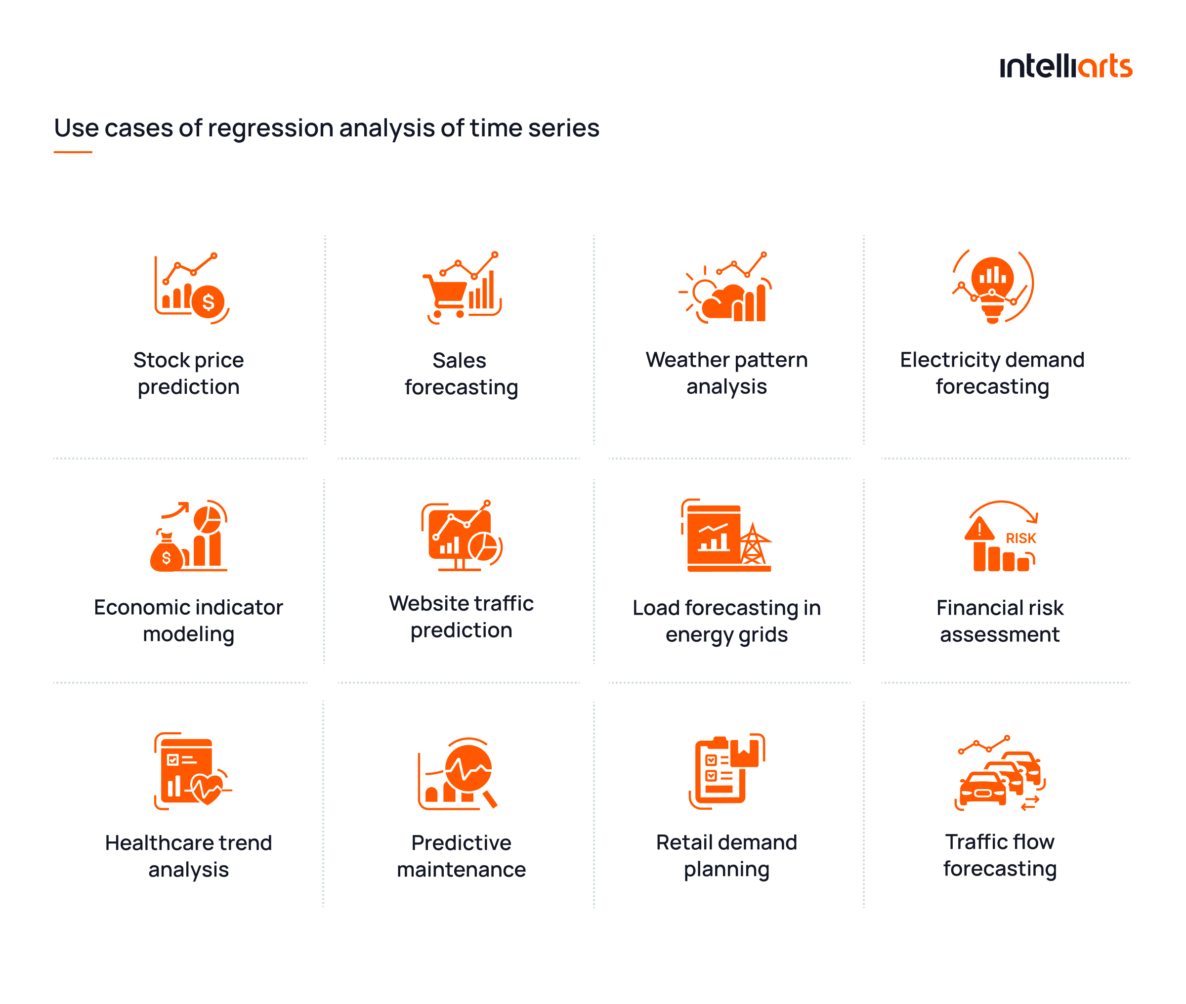
In simple terms, regression analysis with time series data helps you understand how one thing changes over time in response to other factors. For example, it can show how sales depend on advertising spend, time of year, or economic trends while also considering patterns like seasonality or momentum from previous time points. More business use cases of regression analysis of time series are provided in the infographics below:

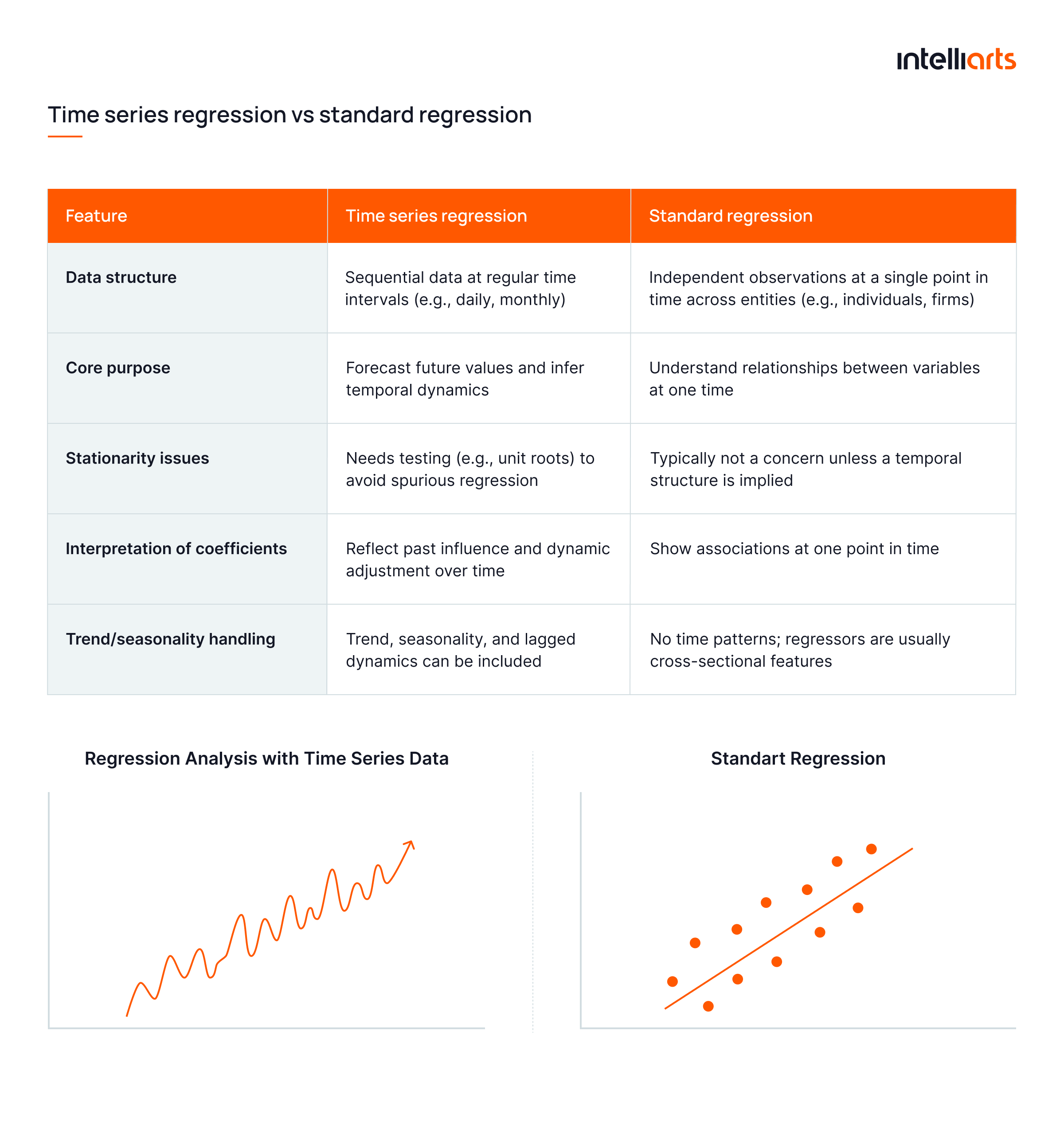
To have a complete picture, let’s compare time series regression analysis to standard regression. 

Standard regression is a statistical method used to examine the relationship between a dependent variable and one or more independent variables, assuming the data points are independent and identically distributed.

Standard regression does not account for time-based patterns, such as trend, seasonality, autocorrelation, etc. That’s what makes this method of analysis suitable for cross-sectional or non-temporal data.

A detailed comparison of these two statistical methods is provided in the table:

How Regression Analysis Works With Time Series Data

Provided that you will likely be using a research analysis tool like Python libraries, Stata, IBM SPSS Statistics, etc., you don’t particularly need to understand the deep technicalities of the process. Alternatively, a dedicated ML and data science team may set up a model, which also doesn’t require in-house knowledge of how regression analysis works at its core.

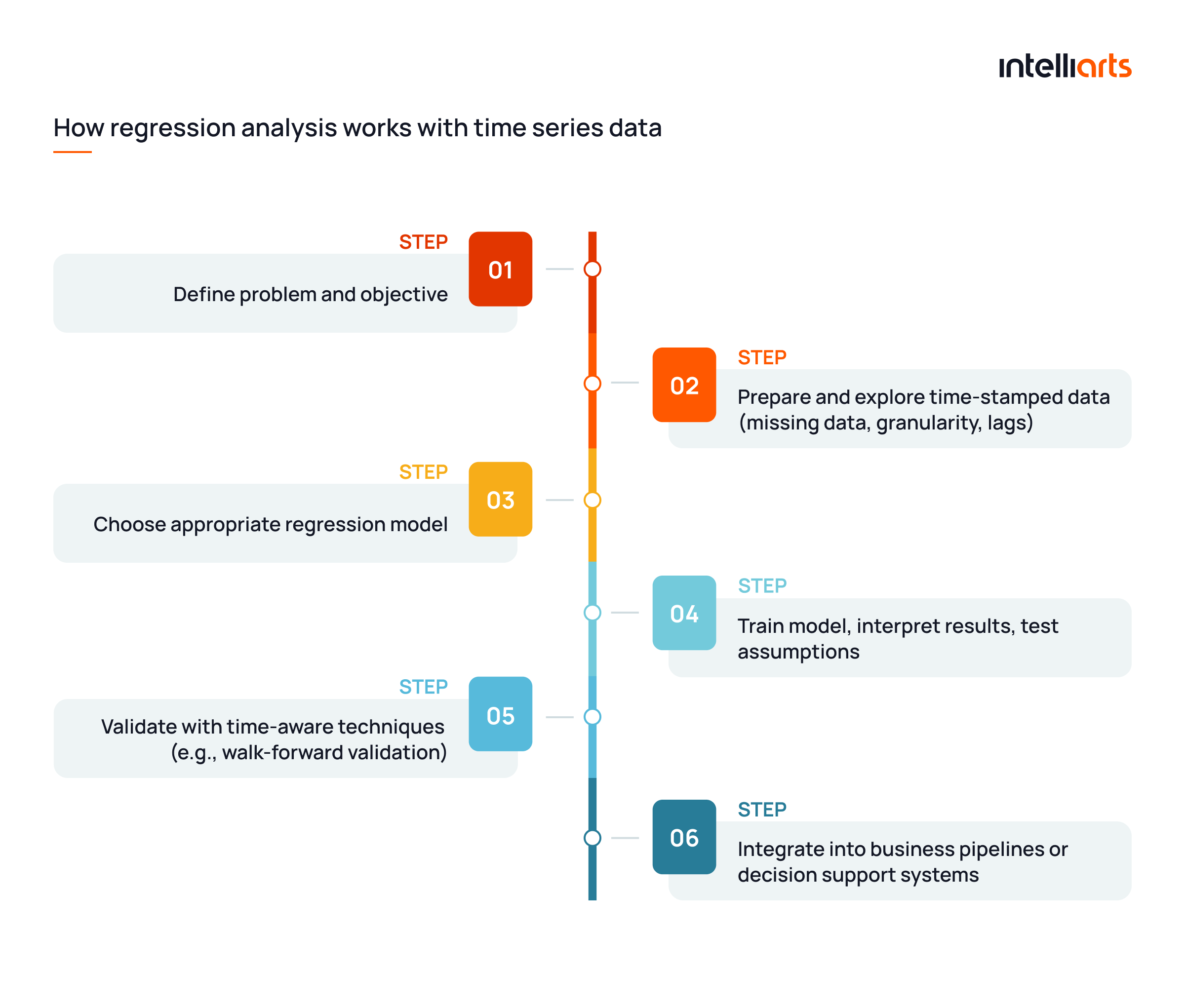
However, knowing how it’s applied in business and how the data in a business project is transformed from a series of numbers into insight is more valuable information. Here it is explained in 6 steps: 

Step 1: Define the Problem and Objective

Clearly state what you want to achieve. Are you forecasting future sales, predicting demand, or analyzing economic trends? To find out, define the following:

• The target variable (e.g., daily sales)
• Independent variables (e.g., marketing spend, day of week)
• The forecasting horizon (e.g., next 30 days)
• Business impact or decisions are dependent on this analysis

Step 2: Prepare and Explore Time-Stamped Data

According to the garbage in, garbage out (GIGO) rule, the accuracy of the analysis largely depends on the quality of the data used for it. To ensure the best possible results, perform the following actions:

• Handling missing data: Fill, interpolate, or drop depending on business context
• Adjusting granularity: Align data to a consistent frequency (e.g., daily, weekly)
• Creating lag features: Include past values of the target or predictors (e.g., sales 1 day ago)
• Exploring trends and seasonality: Visual inspection, decomposition, and plotting are key
• Applying feature engineering if necessary: Time-based features like day of week, month, and holidays

Step 3: Choose an Appropriate Regression Model

Based on data and the initial assumptions about the research, select a model:

• Simple linear regression (with time or lags)
• Autoregressive models (AR) or ARIMAX/ADL (autoregressive with exogenous variables)
• Seasonal models if seasonality is present
• Regularized regressions (Ridge, Lasso) for high-dimensional time-based features

More information on regression analysis forecasting models is provided in the sections below of the blog post. 

“A beautiful aspect of regression analysis is that you hold the other independent variables constant by merely including them in your model!” — Jim Frost, a statistician, author, and data analysis educator

Step 4: Train Model, Interpret Results, Test Assumptions

Fit the model and ensure it meets critical assumptions:

• Linearity between variables
• No autocorrelated residuals (use Durbin-Watson test)
• Homoscedasticity (constant variance of errors)
• Normality of residuals if inference is required

Important: Simple regression analysis can be done using the models listed above and below in the semi-automatic mode. However, complex, fully automated regression analytics using ML and data pipelines should be set up only by qualified ML and data engineers.

Step 5: Validate With Time-Aware Techniques

Traditional cross-validation won’t work due to time dependency. That’s why, when it comes to regression analysis of time series, it’s recommended to do the following:

• Use walk-forward validation, expanding/rolling windows, or time series cross-validation
• Evaluate using metrics like MAE, RMSE, or MAPE that reflect forecast accuracy over time
• Compare against naive models (e.g., last value carried forward) to prove value

Step 6: Integrate Into Business Pipelines or Decision Support Systems

Finally, it’s necessary to make a time series regression model applicable for your business use cases. That’s what ML engineers would do in this stage: 

• Deployment in dashboards, forecasting tools, or automated systems
• Scheduling regular data refresh and retraining
• Building alerts or decision triggers based on predicted values
• Monitoring model drift and performance over time

Practical examples of how companies have used this method to solve actual business issues are provided further in the text. For now, let’s move on to the review of core regression analysis forecasting models. 

Core Regression Models for Time Series Analysis

While models for regression analysis of time series are numerous, let’s focus on the five that are most frequently used. Most likely, you won’t have to actually apply formulas to your datasets yourself, as tools for research analysis are semi-automated, and ML solutions for these purposes are automated. Still, understanding the principles of models that your business data may be accessed through might be helpful. 

1. Linear Regression

What it is: A basic model that assumes a linear relationship between one dependent variable and one or more independent variables over time.

How it works: Estimates coefficients that minimize the squared differences between actual and predicted values. Time is often included as a variable, but autocorrelation and temporal structure are not directly modeled.

Formula: Yₜ = β₀ + β₁Xₜ + εₜ

Where it is used: Short-term forecasting, baseline models, trend estimation, and business metrics tracking, where relationships are stable and simple.

2. Polynomial Regression

What it is: An extension of linear regression that models non-linear relationships using powers of the independent variable(s).

How it works: Transforms the input variable(s) into higher-degree polynomials to capture curves in the data. Useful when the trend is non-linear over time.

Formula: Yₜ = β₀ + β₁Xₜ + β₂Xₜ² + … + βₙXₜⁿ + εₜ

Where it is used: Modeling curvilinear trends, such as growth followed by decay or saturation in economics, population modeling, and market lifecycle curves.

“All models are wrong, but some are useful.” — George E. P. Box, a statistician

3. Multivariate (Multiple) Regression

What it is: A regression that models the relationship between a single time-dependent outcome and multiple independent variables.

How it works: Incorporates multiple predictors (e.g., price, season, weather) at the same time. Assumes independence across observations unless extended for time structure.

Formula: Yₜ = β₀ + β₁X₁ₜ + β₂X₂ₜ + … + βₖXₖₜ + εₜ

Where it is used: Used in demand forecasting, retail sales analysis, energy consumption modeling, and advertising impact studies.

4. Autoregressive Distributed Lag (ADL) Model

What it is: A model that combines past values of the dependent variable (autoregressive terms) with current and lagged values of explanatory variables (distributed lags).

How it works: Captures both internal momentum (e.g., Y depends on past Y) and external effects (e.g., X values over several time lags) in one framework.

Formula: Yₜ = α + φ₁Yₜ₋₁ + φ₂Yₜ₋₂ + … + φₚYₜ₋ₚ + β₀Xₜ + β₁Xₜ₋₁ + … + β_qXₜ₋_q + εₜ

Where it is used: Macroeconomic modeling, energy demand prediction, finance, and any domain where lagged interactions are expected.

5. ARIMA With Exogenous Variables (ARIMAX)

What it is: An ARIMA model extended with external regressors (exogenous variables) that influence the forecast alongside autoregressive and moving average terms.

How it works technically: Integrates three components, autoregression (AR), differencing for stationarity (I), and moving average (MA), plus external inputs (X variables). Useful when both internal dynamics and external drivers matter.

Formula: Yₜ = φ(L)(1 – L)ᵈYₜ + θ(L)εₜ + βXₜ

Where it is used: Forecasting sales with promotions, economic forecasting with interest rates, weather-influenced load forecasting, and financial modeling.

5 Strategies to Interpret and Validate Time Series Regression Results

Without further ado, here are proven tips and strategies that will help you achieve better regression analysis results. Alternatively, use these bits of advice to validate the outcomes of making custom regression models by ML engineers: 

1. Check Residuals Over Time

Plot residuals to see if errors are randomly distributed. Patterns may indicate missing variables or model misspecification. That’s why it’s essential to use ACF plots of residuals to detect autocorrelation.

2. Compare Forecast Accuracy

Use time-aware metrics like MAE, RMSE, or MAPE. Benchmark against naive models (e.g., last period value). Consistently better performance validates the model's usefulness.

3. Assess Coefficient Stability

Review signs and significance across rolling windows or retrained models. Inconsistent coefficients may suggest overfitting or non-stationary effects. Stability implies reliable long-term relationships.

4. Monitor Out-of-Sample Performance

Split the data chronologically and test on future periods. Walk-forward validation reveals how the model handles real forecasting conditions. Poor generalization indicates a need for refinement.

5. Align Results With Business Context

Interpret findings in terms of known cycles, events, or policies. Validate with domain experts to ensure insights are realistic. If results contradict expectations, reassess assumptions or features.

Final Take

Time series regression helps uncover how variables evolve over time, accounting for trends, seasonality, and lagged relationships. Models like linear, polynomial, ADL, or ARIMAX enable accurate forecasting in areas where timing matters, such as inventory planning, promotions, or economic analysis. Reliable results depend on well-prepared data, time-aware validation, and model stability, making this method a practical choice for businesses working with temporal data.