A Very Basic Introduction to Feed-Forward Neural Networks
Don't have a clue about feed-forward neural networks? No problem! Read on for an example of a simple neural network to understand its architecture, math, and layers.
Join the DZone community and get the full member experience.
Join For FreeBefore we get started with our tutorial, let's cover some general terminology that we'll need to know.
General Architecture
Node: The basic unit of computation (represented by a single circle)
Layer: A collection of nodes of the same type and index (i.e. input, hidden, outer layer)
Connection: A weighted relationship between a node of one layer to the node of another layer
W: The weight of a connection
I: Input node (the neural network input)
H: Hidden node (a weighted sum of input layers or previous hidden layers)
HA: Hidden node activated (the value of the hidden node passed to a predefined function)
O: Outut node (A weighted sum of the last hidden layer)
OA: Output node activated (the neural network output, the value of an output node passed to a predefined function)
B: Bias node (always a contrant, typically set equal to 1.0)
e: Total difference between the output of the network and the desired value(s) (total error is typically measured by estimators such as mean squared error, entropy, etc.)
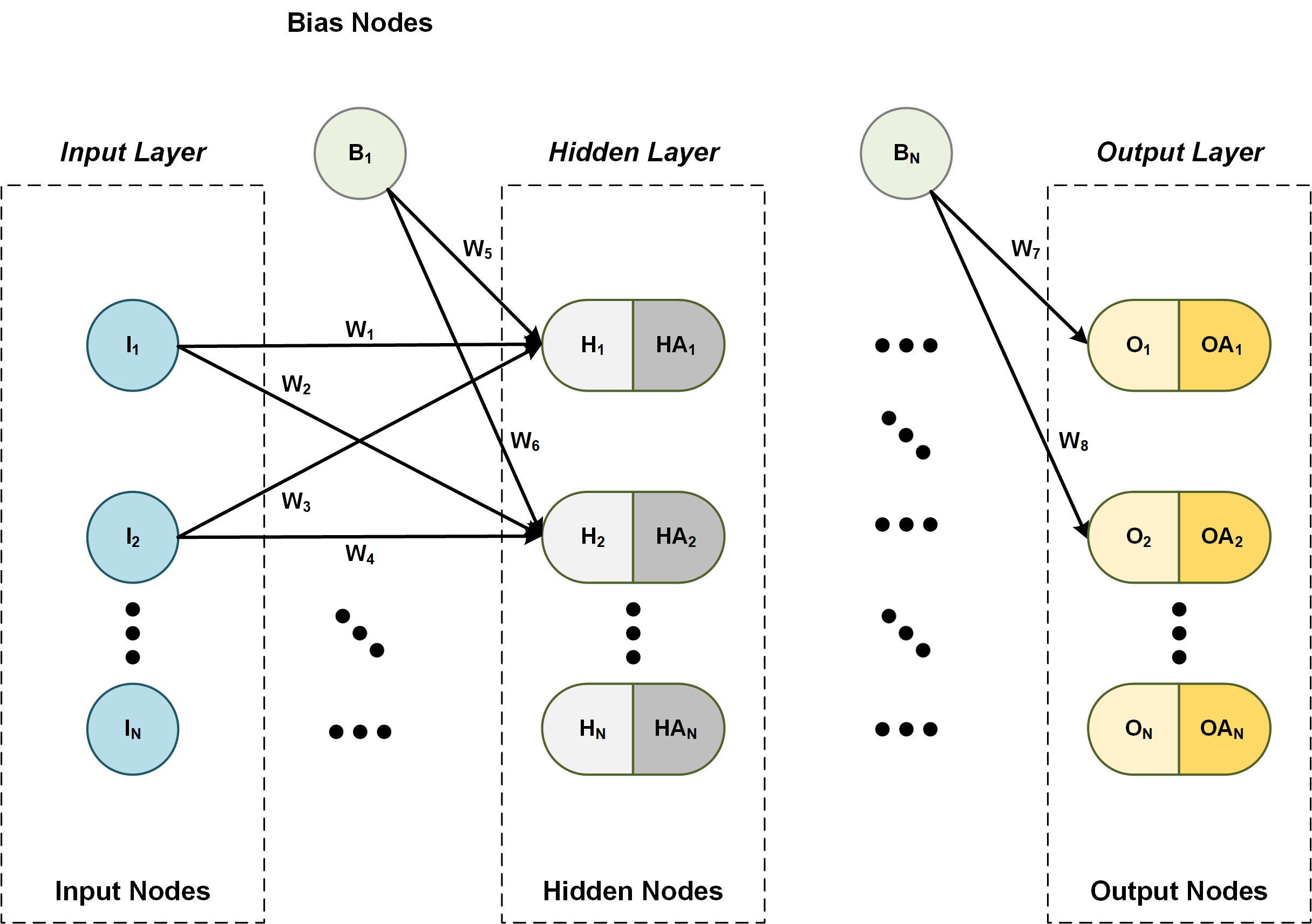
Figure 1: General architecture of a neural network
Getting straight to the point, neural network layers are independent of each other; hence, a specific layer can have an arbitrary number of nodes. Typically, the number of hidden nodes must be greater than the number of input nodes. When the neural network is used as a function approximation, the network will generally have one input and one output node. When the neural network is used as a classifier, the input and output nodes will match the input features and output classes. A neural network must have at least one hidden layer but can have as many as necessary. The bias nodes are always set equal to one. In analogy, the bias nodes are similar to the offset in linear regression i.e. y = mx+b. How does one select the proper number of nodes and hidden number of layers? This is the best part: there are really no rules! The modeler is free to use his or her best judgment on solving a specific problem. Experience has shown that there are best practices such as selecting an adequate number of hidden layers, activation functions, and training methods; however, this is beyond the scope of this article.
As a user, one first has to construct the neural network, then train the network by iterating with known outputs (AKA desired output, expected values) until convergence, and finally, use the trained network for prediction, classification, etc.
The Math
Let's consider a simple neural network, as shown below.
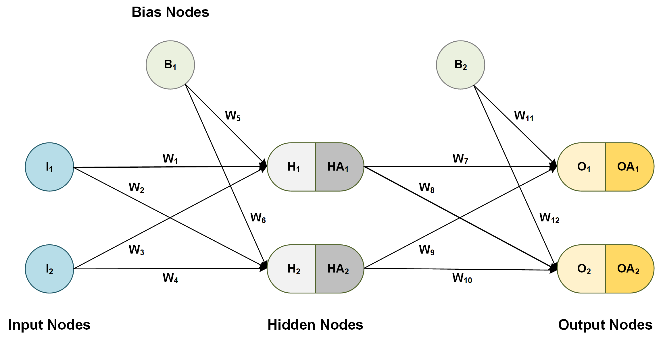
Figure 2: Example of a simple neural network
Step 1: Initialization
The first step after designing a neural network is initialization:
- Initialize all weights W1 through W12 with a random number from a normal distribution, i.e. ~N(0, 1).
- Set all bias nodes B1 = B2 = 1.0.
Note: Keep in mind that the variance of the distribution can be a different value. This has an effect on the convergence of the network.
Step 2: Feed-Forward
As the title describes it, in this step, we calculate and move forward in the network all the values for the hidden layers and output layers.
- Set the values of all input nodes.
- Calculate hidden node values.
- Select an activation function for the hidden layer; for example, the Sigmoid function:

- Calculate hidden node activation values:
- Calculate output node values:
- Select an activation function for the output layer; for example, the linear function:

- Calculate output node activation values:

- Calculate the total error; if OAi is the obtained output value for node i, then let yi be the desired output.
 Note: Here, the error is measured in terms of the mean square error, but the modeler is free to use other measures, such as entropy or even custom loss functions..
After the first pass, the error will be substantial, but we can use an algorithm called backpropagation to adjust the weights to reduce the error between the output of the network and the desired values
Step 3: Backpropagation
This is the step where the magic happens. The goal of this step is to incrementally adjust the weights in order for the network to produce values as close as possible to the expected values from the training data.
Note: Keep in mind statistical principles such as overfitting, etc.
Backpropagation can adjust the network weights using the stochastic gradient decent optimization method.
Where k is the iteration number, η is the learning rate (typically a small number), and:  ...is the derivative of the total error with regards to to the weight adjusted.
In this procedure, we derive a formula for each individual weight in the network, including bias connection weights. The example below shows the derivation of the update formula (gradient) for the first weight in the network.
Let's calculate the derivative of the error e with regards to to a weight between the input and hidden layer, for example, W1 using the calculus chain rule.
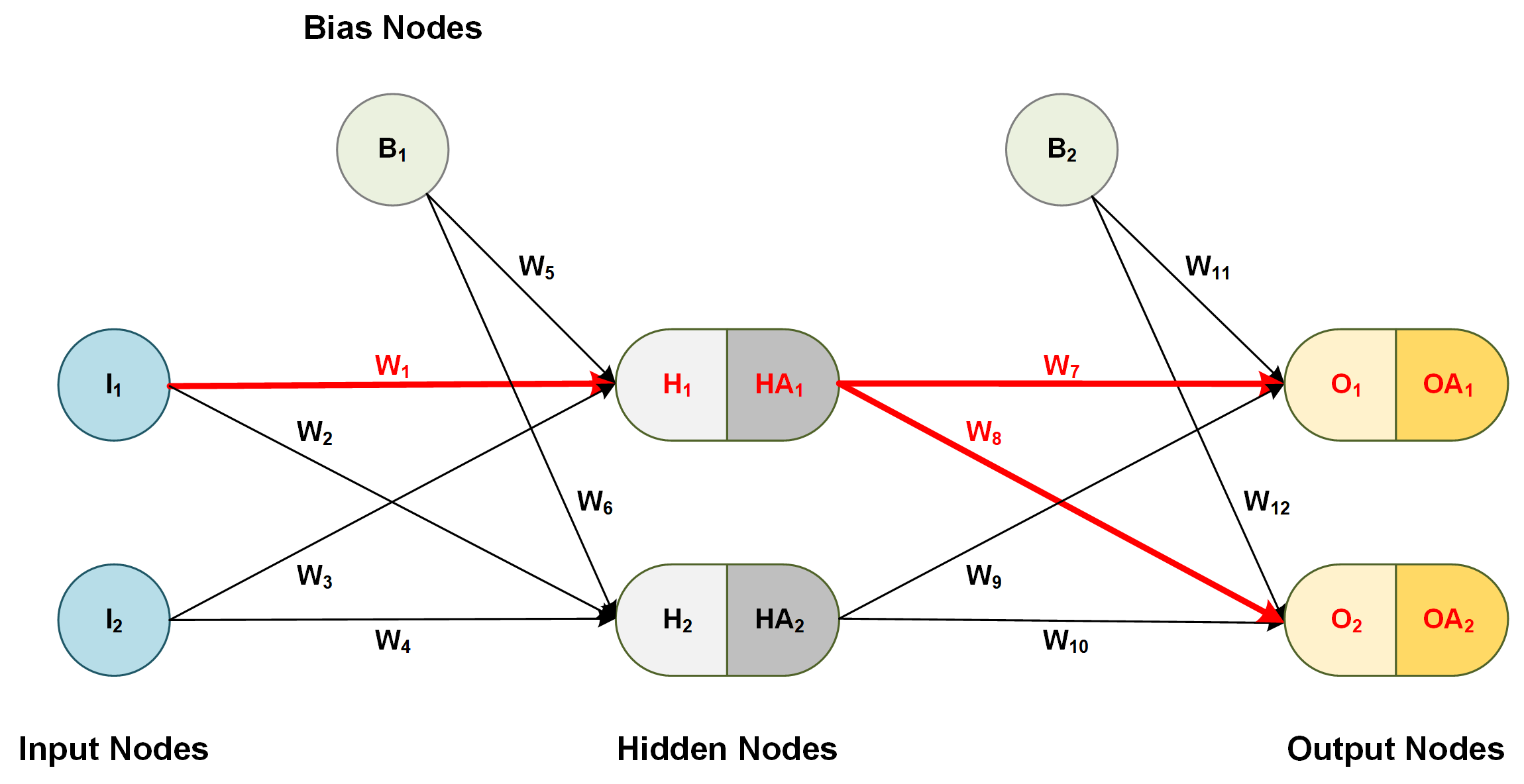
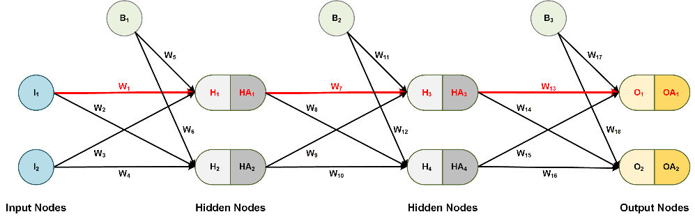
Figure 3: Chain rule for weights between input and hidden layer
- Start from the very first activated output node and take derivatives backward for each node. For simplicity, one can think of a node and its activated self as two different nodes without a connection.
- From the activated output bounce to the output node:
- From the output node bounce to the first activated node of the last hidden layer:
- From the activated hidden node, bounce to the hidden node itself:
- From the first hidden node, bounce to the weight of the first connection:
This concludes one unique path to the weight derivative — but wait... there is one additional path that we have to calculate. Refer to Figure 3, and notice the connections and nodes marked in red.
- Once again, start from the next activated output node and make your way backward by taking derivatives for each node. This time, we do not need to spell out every step.
- Finally, the total derivative for the first weight W1 in our network is the sum of the product the individual node derivatives for each specific path.
Note that we leave out the second hidden node because the first weight in the network does not depend on the node. This is clearly seen in Figure 3 above.
We follow the same procedure for all the weights one-by-one in the network.
Here is another example where we calculate the derivative of the error with regard to a weight between the hidden layer and the output layer:
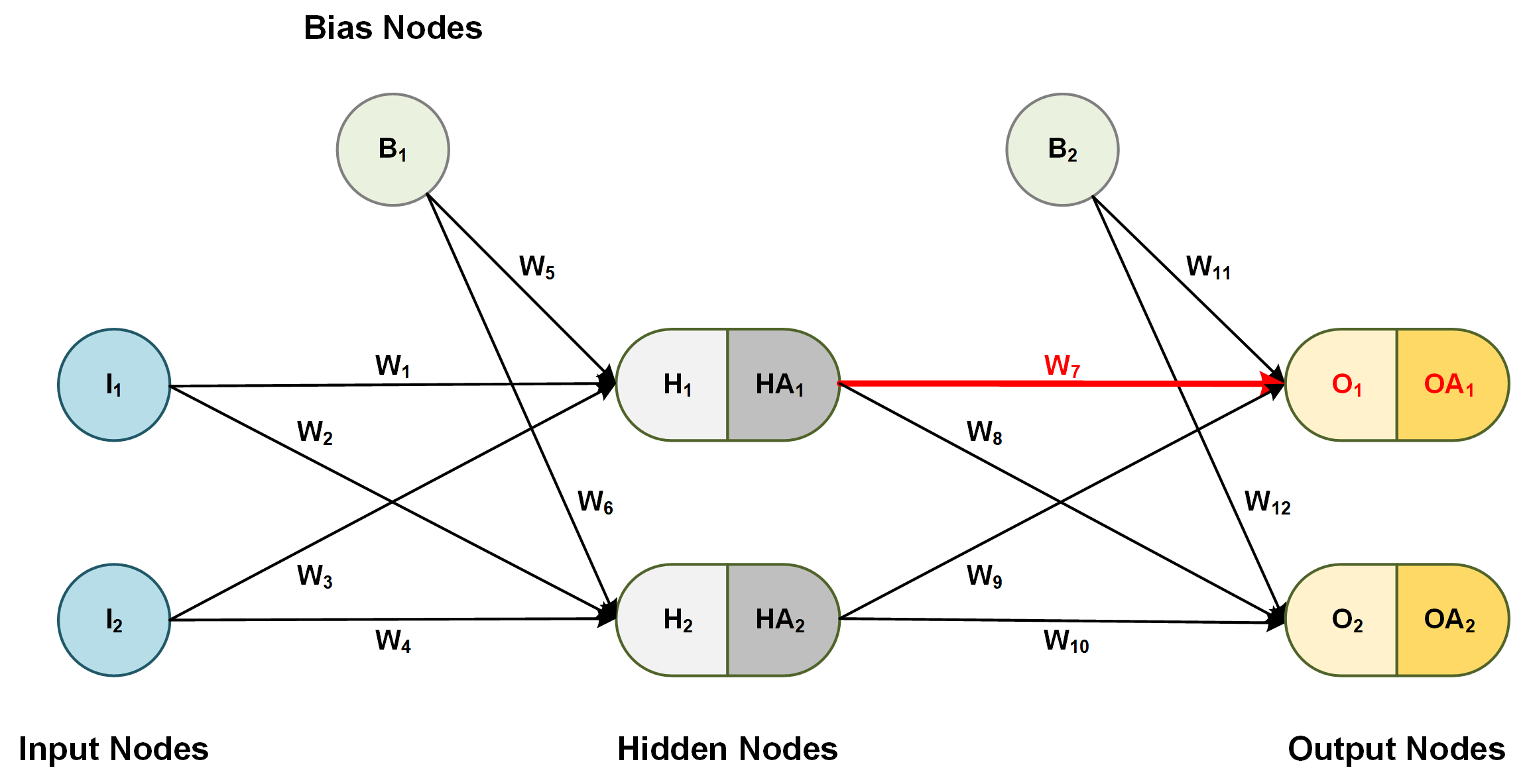
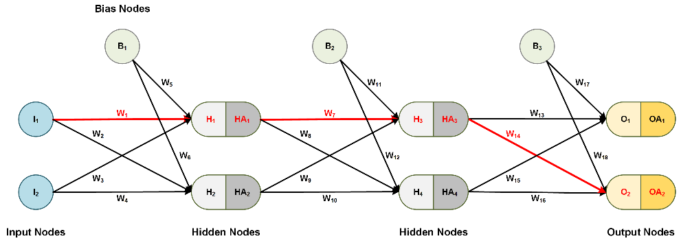
Figure 4: Chain rule for weights between hidden and output layer
- As in the previous step, start with the very first activated output weight in the network and take derivatives backward all the way to the desired weight, and leave out any nodes that do not affect that specific weight:
- Lastly, we take the sum of the product of the individual derivatives to calculate the formula for the specific weight:
The same strategy applies to bias weights.
Once we have calculated the derivatives for all weights in the network (derivatives equal gradients), we can simultaneously update all the weights in the net with the gradient decent formula, as shown below.
Notes: Calculus Chain Rule
Why do we calculate derivatives for all these unique paths? Note that the backpropagation is a direct application of the calculus chain rule.
For example:
- Let's define the following functions:

- If we need to take the derivate of z with regard to t, then by the calculus chain rule, we have:
Note that the total derivative of z with regard to t is the sum of the product of the individual derivatives. What if t is also a function of another variable?
- Let's define another function:

- Then, the derivate of z with respect to s, by the calculus chain rule, is the following:
Now, let's compare the chain rule with our neural network example and see if we can spot a pattern.
- Let's borrow the follow functions from our neural network example:
- If we need to take the derivate of e, with respect to HA1, then by the chain rule, we have:
The same pattern follows if HA1 is a function of another variable.
At this point, it should be clear that the backpropagation is nothing more than the direct application of the calculus chains rule. One can identify the unique paths to a specific weight and take the sum of the product of the individual derivatives all the way to a specific weight.
Note: If you understand everything thus far, then you understand feedforward multilayer neural networks.
Deep Neural Networks
Two Hidden Layers
Neural networks with two or more hidden layers are called deep networks. The same rules apply as in the simpler case; however, the chain rule is a bit longer.
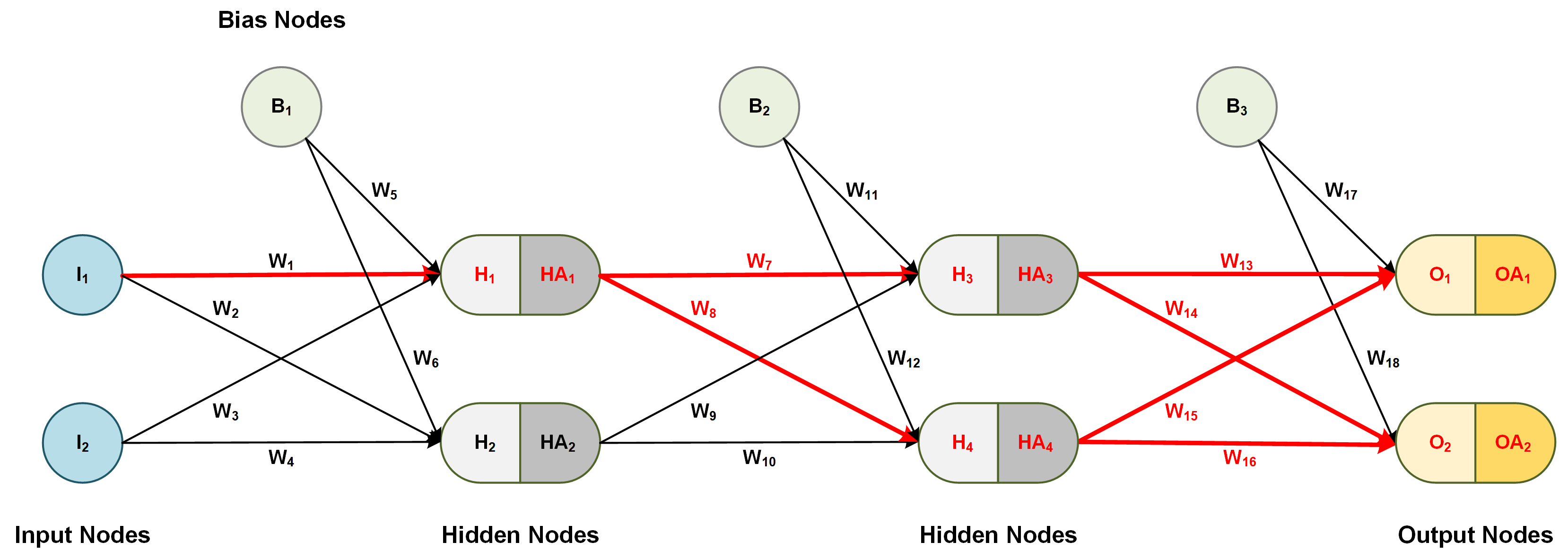
Figure 5: Chain rule for weights between input and hidden layer
As an example, let's reevaluate the total derivative of the error with regard to W1, which is the sum of the product of each unique path from each output node, i.e. the sum of the products (paths 1-4).
See example paths below.


- Next, we can factor the common terms, and the total derivative for W1 is complete!
Notice something interesting here: each product factor belongs to a different layer. This observation will be useful later in the formulation.
Three Hidden Layers
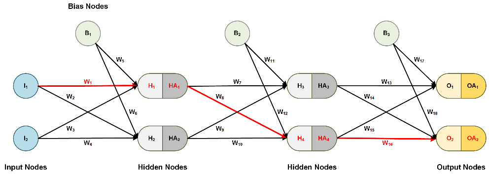
Yet another example of a deep neural network with three hidden layers:
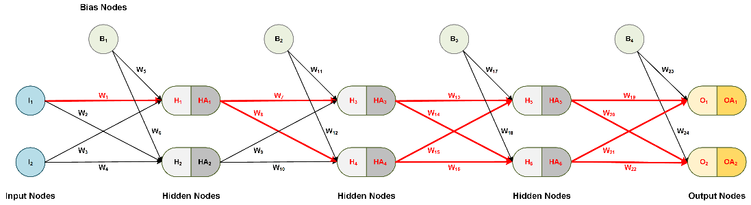
Figure 6: Chain rule for weights between input and hidden layer
Once again, the total derivative of the error e with regard to W1 is the sum of the product of all paths (paths 1-8). Note that there are more path combinations with more hidden layers and nodes per layer.
- And again, we factor the common terms and re-write the equation below:
Pattern
To efficiently program a structure, perhaps there exists some pattern where we can reuse the calculated partial derivatives.
To illustrate the pattern, let's observe the total derivatives for W1, W7, W13, and W19 in Figure 6 above. Note that these are not all the weights in the net but they are sufficient to make the point.
We can view the factored total derivatives for the specified weights in a tree-like form as shown below.
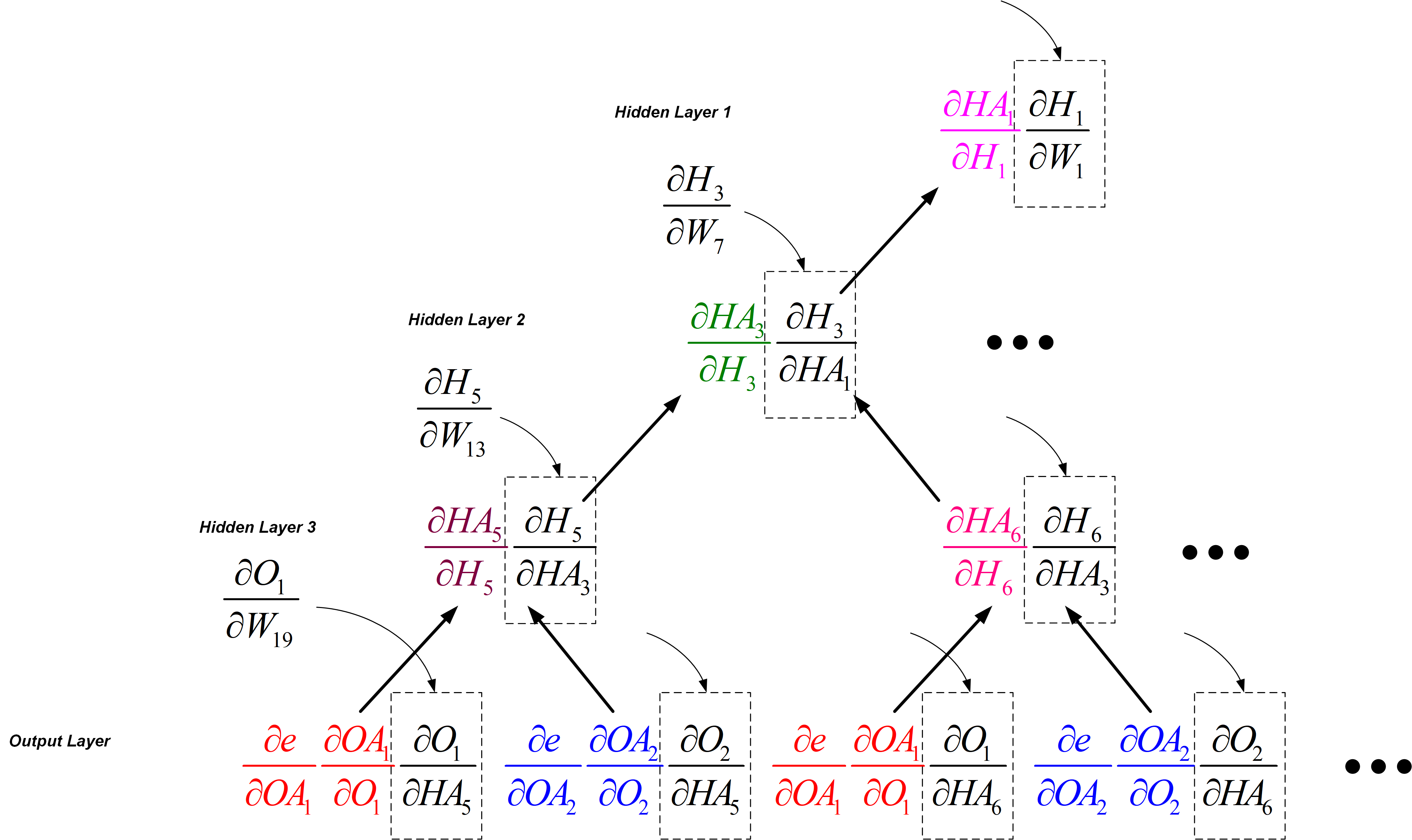
The rule to find the total derivative for a particular weight is to add the tree leaves in the same layer and multiply leaves up the branch.
For example, to find the total derivative for W7 in Hidden Layer 2, we can replace (dH3/dHA1) with (dH3/dW13) and we obtain the correct formula. Note: We ignore the higher terms in Hidden Layer 1.
We can do the same for W13, W19, and all other weight derivatives in the network by adding the lower level leaves, multiplying up the branch, replacing the correct partial derivative, and ignoring the higher terms.
The advantage of this structure is that one can pre-calculate all the individual derivatives and then, use summation and multiplication as less expensive operations to train the neural network using backpropagation.
Hope this helps!
Published at DZone with permission of Edvin Beqari. See the original article here.
Opinions expressed by DZone contributors are their own.
Comments