Understanding Index Grouping and Aggregation in Couchbase N1QL Queries

Couchbase N1QL is a modern query processing engine designed to provide SQL for JSON on distributed data with a flexible data model. Modern databases are deployed on massive clusters. Using JSON provides a flexible data model. N1QL supports enhanced SQL for JSON to make query processing easier.

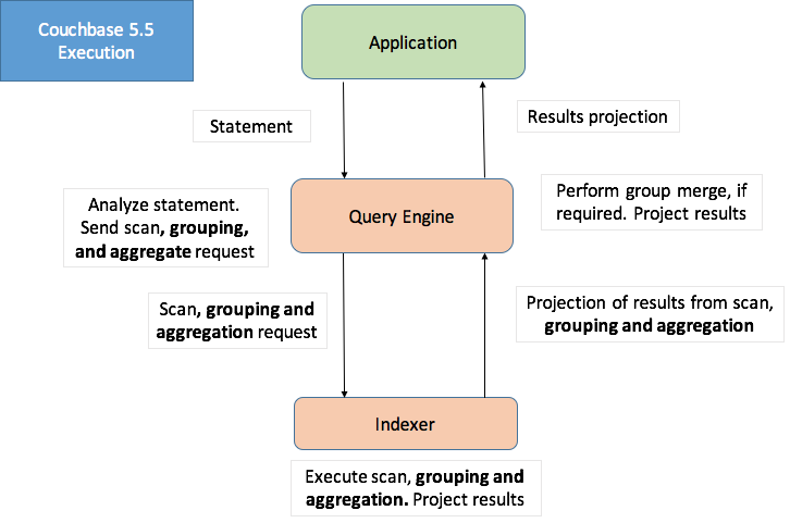
Applications and database drivers submit the N1QL query to one of the available Query nodes on a cluster. The Query node analyzes the query and uses metadata on underlying objects to figure out the optimal execution plan, which it then executes. During execution, depending on the query, when using applicable indexes, the Query node works with index and data nodes to retrieve data and perform the planned operations. Because Couchbase is a modular clustered database, you scale out data, index, and query services to fit your performance and availability goals.

Prior to Couchbase 5.5, even when a query with GROUP BY and/or aggregates is covered by an index, the query fetched all relevant data from the indexer and performed grouping/aggregation of the data within the query engine.

In Couchbase 5.5, Query Planner was enhanced to intelligently request the indexer to perform grouping and aggregation in addition to range scan for covering index. The indexer has been enhanced to perform grouping, COUNT(), SUM(), MIN(), MAX(), AVG(), and related operations on the fly.

This requires no changes to the user query, but a good index design to cover the query and order the index keys is required. Not every query will benefit from this optimization, and not every index can accelerate every grouping and aggregation operation. Understanding the right patterns will help you design your indexes and queries. Index grouping and aggregation on global secondary indexes is supported with both storage engines: standard GSI and memory-optimized GSI (MOI). Index grouping and aggregation is supported in the Enterprise Edition only.

This reduction step of performing the GROUP BY and Aggregation by the indexer reduces the amount of data transfer and disk I/O, resulting in:

• Improved query response time
• Improved resource utilization
• Low latency
• High scalability
• Low total cost of ownership

Performance

The Index grouping and aggregations can improve query performance by orders of magnitude and reduce latency drastically. The following table lists a few sample query latency measurements.

Index:

CREATE INDEX idx_ts_type_country_city ON `travel-sample` (type, country, city);

Index Grouping and Aggregation Overview

The above figure shows all the possible phases that a SELECT query goes through to return the results. The filtering process takes the initial keyspace and produces an optimal subset of the documents the query is interested in. To produce the smallest possible subset, indexes are used to apply as many predicates as possible. The query predicate indicates the subset of the data interested. During the query planning phase, we select the indexes to be used. Then, for each index, we decide the predicates to be applied by each index. The query predicates are translated into range scans in the query plan and passed to Indexer.

If the query doesn't have JOINs and is covered by index, both Fetch and Join phases can be eliminated.

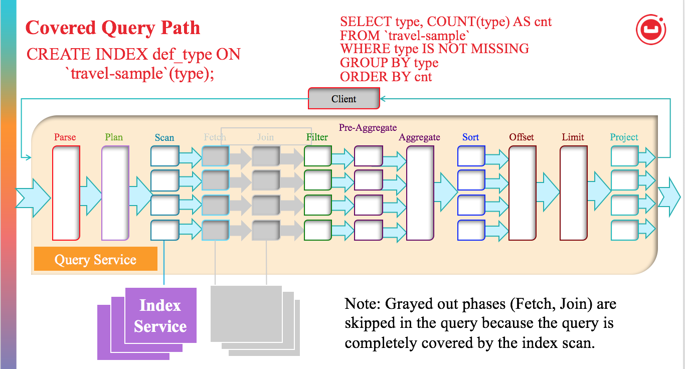
When all predicates are exactly translated to range scans, the Filter phase also can be eliminated. In that situation, Scan and Aggregates are side-by-side, and since Indexer has the ability to do aggregation, that phase can be done on indexer node. In some cases, Sort, Offset, and Limit phases can also be done on the Indexer node.

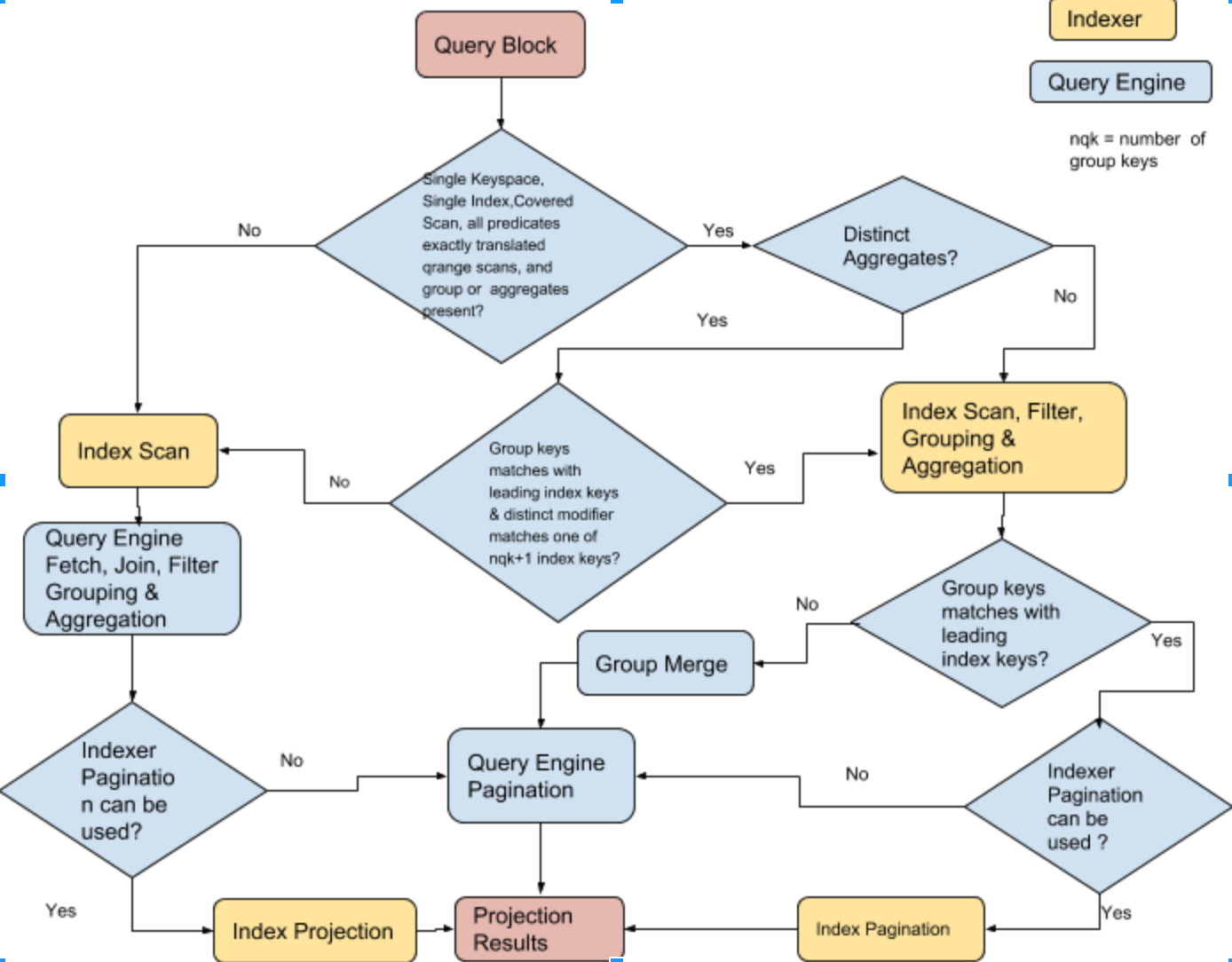
The following flowchart describes how Query Planner decides to perform index aggregation for each query block of the query. If the index aggregation is not possible, aggregations are done in Query Engine.

For example, let's compare the previous vs. current performance of using GROUP BY and examine the EXPLAIN plan of the following query that uses an index defined on the Couchbase travel-sample bucket:

CREATE INDEX `def_type` ON `travel-sample`(`type`);

Consider the query:

SELECT type, COUNT(type)
FROM `travel-sample`
WHERE type IS NOT MISSING
GROUP BY type;

Before Couchbase version 5.5, this query engine fetched relevant data from the indexer and grouping and aggregation of the data is done within query engine. This simple query takes about 250 ms.

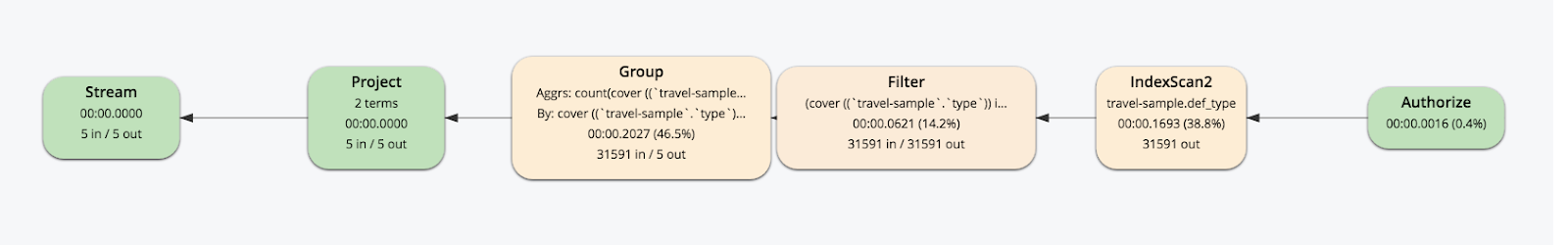
Now, in Couchbase version 5.5, this query uses the same def_type index but executes in under 20 ms. In the explanation below, you can see fewer steps and the lack of the grouping step after the index scan because the index scan step does the grouping and aggregation, as well.

As the data and query complexity grows, the performance benefit (both latency and throughput) will grow as well.

Understanding EXPLAIN of Index Grouping and Aggregation

Looking at the explanation of the query:

EXPLAIN SELECT type, COUNT(type) FROM `travel-sample` WHERE type IS NOT MISSING GROUP BY type;

{
  "plan": {
    "#operator": "Sequence",
    "~children": [
      {
        "#operator": "IndexScan3",
        "covers": [
          "cover ((`travel-sample`.`type`))",
          "cover ((meta(`travel-sample`).`id`))",
          "cover (count(cover ((`travel-sample`.`type`))))"
        ],
        "index": "def_type",
        "index_group_aggs": {
          "aggregates": [
            {
              "aggregate": "COUNT",
              "depends": [
                0
              ],
              "expr": "cover ((`travel-sample`.`type`))",
              "id": 2,
              "keypos": 0
            }
          ],
          "depends": [
            0
          ],
          "group": [
            {
              "depends": [
                0
              ],
              "expr": "cover ((`travel-sample`.`type`))",
              "id": 0,
              "keypos": 0
            }
          ]
        },
        "index_id": "b948c92b44c2739f",
        "index_projection": {
          "entry_keys": [
            0,
            2
          ]
        },
        "keyspace": "travel-sample",
        "namespace": "default",
        "spans": [
          {
            "exact": true,
            "range": [
              {
                "inclusion": 1,
                "low": "null"
              }
            ]
          }
        ],
        "using": "gsi"
      },
      {
        "#operator": "Parallel",
        "~child": {
          "#operator": "Sequence",
          "~children": [
            {
              "#operator": "InitialProject",
              "result_terms": [
                {
                  "expr": "cover ((`travel-sample`.`type`))"
                },
                {
                  "expr": "cover (count(cover ((`travel-sample`.`type`))))"
                }
              ]
            },
            {
              "#operator": "FinalProject"
            }
          ]
        }
      }
    ]
  },
  "text": "SELECT type, COUNT(type) FROM `travel-sample` WHERE type IS NOT MISSING GROUP BY type;"
}

You will see index_group_aggs in the IndexScan section (i.e "#operator": "IndexScan3"). If index_group_aggs is missing, then the query service is performing grouping and aggregation. If it's present,the query is using Index grouping and aggregation and it has all relevant information indexer required for grouping and aggregation. The following table describes how to interpret the various information of the index_group_aggs object.

The covers field is an array and it has all the index keys, document keys (META().id), group keys expressions that are not exactly matched with index keys (sorted by ID), and aggregates sorted by ID. Also, Index_projection will have all the group/aggregate IDs.

"covers": [

"cover ((`travel-sample`.`type`))", ← Index key (0)

"cover ((meta(`travel-sample`).`id`))", ← document key (1)

"cover (count(cover ((`travel-sample`.`type`))))" ← aggregate (2)

]

In the above case, the group expression type is the same Index key of index def_type. It is not included twice.

Details of Index Grouping and Aggregation

We will use examples to show how index grouping and aggregation work. To follow the examples, please create a bucket default and insert the following documents:

INSERT INTO default (KEY,VALUE) 
VALUES ("ga0001", {"c0":1, "c1":10, "c2":100, "c3":1000, "c4":10000, "a1":[{"id":1}, {"id":1}, {"id":2}, {"id":3}, {"id":4}, {"id":5}]}),
VALUES ("ga0002", {"c0":1, "c1":20, "c2":200, "c3":2000, "c4":20000, "a1":[{"id":1}, {"id":1}, {"id":2}, {"id":3}, {"id":4}, {"id":5}]}),
VALUES ("ga0003", {"c0":1, "c1":10, "c2":300, "c3":3000, "c4":30000, "a1":[{"id":1}, {"id":1}, {"id":2}, {"id":3}, {"id":4}, {"id":5}]}),
VALUES ("ga0004", {"c0":1, "c1":20, "c2":400, "c3":4000, "c4":40000, "a1":[{"id":1}, {"id":1}, {"id":2}, {"id":3}, {"id":4}, {"id":5}]}),
VALUES ("ga0005", {"c0":2, "c1":10, "c2":100, "c3":5000, "c4":50000, "a1":[{"id":1}, {"id":1}, {"id":2}, {"id":3}, {"id":4}, {"id":5}]}),
VALUES ("ga0006", {"c0":2, "c1":20, "c2":200, "c3":6000, "c4":60000, "a1":[{"id":1}, {"id":1}, {"id":2}, {"id":3}, {"id":4}, {"id":5}]}),
VALUES ("ga0007", {"c0":2, "c1":10, "c2":300, "c3":7000, "c4":70000, "a1":[{"id":1}, {"id":1}, {"id":2}, {"id":3}, {"id":4}, {"id":5}]}),
VALUES ("ga0008", {"c0":2, "c1":20, "c2":400, "c3":8000, "c4":80000, "a1":[{"id":1}, {"id":1}, {"id":2}, {"id":3}, {"id":4}, {"id":5}]});

Example 1: Group by Leading Index Keys

Let's consider the following query and index:

SELECT d.c0 AS c0, d.c1 AS c1, SUM(d.c3) AS sumc3, 
        AVG(d.c4) AS avgc4, COUNT(DISTINCT d.c2) AS dcountc2
FROM default AS d
WHERE d.c0 > 0
GROUP BY d.c0, d.c1
ORDER BY d.c0, d.c1
OFFSET 1 
LIMIT 2;

Required index:

CREATE INDEX idx1 ON default(c0,c1,c2,c3,c4);

The query has GROUP BY and multiple aggregates, and some aggregates have a DISTINCT modifier. The query can be covered by index idx1 and the predicate (d.c0 > 0) can be converted into exact range scan and pass it to index scan. So, the index and query combination qualifies index grouping and aggregations.

Indexes are naturally ordered and grouped by the order of the index key definition. In the above query, the GROUP BY keys (d.c0, d.c1) exactly match the leading keys (c0, c1) of the index. Therefore, the index has each group data together and the indexer will produce one row per group, i.e. full aggregation. Also, the query has an aggregate that has a DISTINCT modifier and it exactly matches with one of the index keys with position less than or equal to number of group keys plus one (i.e. there two group keys, so the DISTINCT modifier can be any one of an index key at position 0, 1, or 2 because the index key followed by group keys and DISTINCT modifier can be applied without sort). Therefore, the query above is suitable for the indexer to handle grouping and aggregation.

If GROUP BY is missing one of the leading index keys and there is equality predicate, then special optimization is done by treating the index key implicitly present in group keys and determine if full aggregation is possible. For partition indexing, the all the partition keys need to present in the group keys to generate full aggregations.

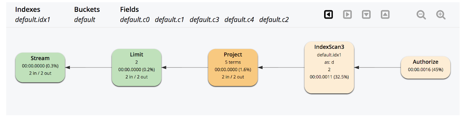
The above graphical execution tree shows index scan (IndexScan3) performing scan and index grouping aggregations. The results from the index scan are projected.

Let's look at the text-based explanation:

{
  "plan": {
    "#operator": "Sequence",
    "~children": [
      {
        "#operator": "Sequence",
        "~children": [
          {
            "#operator": "IndexScan3",
            "as": "d",
            "covers": [
              "cover ((`d`.`c0`))",
              "cover ((`d`.`c1`))",
              "cover ((`d`.`c2`))",
              "cover ((`d`.`c3`))",
              "cover ((`d`.`c4`))",
              "cover ((meta(`d`).`id`))",
              "cover (count(distinct cover ((`d`.`c2`))))",
              "cover (countn(cover ((`d`.`c4`))))",
              "cover (sum(cover ((`d`.`c3`))))",
              "cover (sum(cover ((`d`.`c4`))))"
            ],
            "index": "idx1",
            "index_group_aggs": {
              "aggregates": [
                {
                  "aggregate": "COUNT",
                  "depends": [
                    2
                  ],
                  "distinct": true,
                  "expr": "cover ((`d`.`c2`))",
                  "id": 6,
                  "keypos": 2
                },
                {
                  "aggregate": "COUNTN",
                  "depends": [
                    4
                  ],
                  "expr": "cover ((`d`.`c4`))",
                  "id": 7,
                  "keypos": 4
                },
                {
                  "aggregate": "SUM",
                  "depends": [
                    3
                  ],
                  "expr": "cover ((`d`.`c3`))",
                  "id": 8,
                  "keypos": 3
                },
                {
                  "aggregate": "SUM",
                  "depends": [
                    4
                  ],
                  "expr": "cover ((`d`.`c4`))",
                  "id": 9,
                  "keypos": 4
                }
              ],
              "depends": [
                0,
                1,
                2,
                3,
                4
              ],
              "group": [
                {
                  "depends": [
                    0
                  ],
                  "expr": "cover ((`d`.`c0`))",
                  "id": 0,
                  "keypos": 0
                },
                {
                  "depends": [
                    1
                  ],
                  "expr": "cover ((`d`.`c1`))",
                  "id": 1,
                  "keypos": 1
                }
              ]
            },
            "index_id": "d06df7c5d379cd5",
            "index_order": [
              {
                "keypos": 0
              },
              {
                "keypos": 1
              }
            ],
            "index_projection": {
              "entry_keys": [
                0,
                1,
                6,
                7,
                8,
                9
              ]
            },
            "keyspace": "default",
            "limit": "2",
            "namespace": "default",
            "offset": "1",
            "spans": [
              {
                "exact": true,
                "range": [
                  {
                    "inclusion": 0,
                    "low": "0"
                  }
                ]
              }
            ],
            "using": "gsi"
          },
          {
            "#operator": "Parallel",
            "maxParallelism": 1,
            "~child": {
              "#operator": "Sequence",
              "~children": [
                {
                  "#operator": "InitialProject",
                  "result_terms": [
                    {
                      "as": "c0",
                      "expr": "cover ((`d`.`c0`))"
                    },
                    {
                      "as": "c1",
                      "expr": "cover ((`d`.`c1`))"
                    },
                    {
                      "as": "sumc3",
                      "expr": "cover (sum(cover ((`d`.`c3`))))"
                    },
                    {
                      "as": "avgc4",
                      "expr": "(cover (sum(cover ((`d`.`c4`)))) / cover (countn(cover ((`d`.`c4`)))))"
                    },
                    {
                      "as": "dcountc2",
                      "expr": "cover (count(distinct cover ((`d`.`c2`))))"
                    }
                  ]
                },
                {
                  "#operator": "FinalProject"
                }
              ]
            }
          }
        ]
      },
      {
        "#operator": "Limit",
        "expr": "2"
      }
    ]
  },
  "text": "SELECT d.c0 AS c0, d.c1 AS c1, SUM(d.c3) AS sumc3, AVG(d.c4) AS avgc4, COUNT(DISTINCT d.c2) AS dcountc2 FROM default AS d\nWHERE d.c0 > 0 GROUP BY d.c0, d.c1 ORDER BY d.c0, d.c1 OFFSET 1  LIMIT 2;"
}

• The index_group_aggs (lines 24-89) in the IndexScan section (i.e "#operator": "IndexScan3") shows a query using index grouping and aggregations.
• If a query uses index grouping and aggregation, the predicates are exactly converted to range scans and passed to the index scan as part of spans, so there will not be any filter operator in the explain.
• As GROUP BY keys exactly match the leading index keys, the indexer will produce full aggregations. Therefore, we also eliminate grouping in query service (there are no InitialGroup, IntermediateGroup, or FinalGroup operators in the explanation).
• Indexer projects index_projection (lines 99-107), including all group keys and aggregates.
• Query ORDER BY matches with leading index keys, and when GROUP BY is on leading index keys, we can use index order. This can be found in the explanation (lines 91-98) and will not use "#operator": "Order" between lines 164-165.
• As the query can use index order and there is no HAVING clause in the query, the offset and limit values can be passed to the indexer.
• This can be found at lines 112 and 110. The offset can be applied only once, so you will not see "#operator": "Offset" between lines 164-165, but re-applying limit is a no. This can be seen at lines 165-168.
• Query contains AVG(x) and it has been rewritten as SUM(x)/COUNTN(x). The COUNTN(x) only counts when x is a numerical value.

Example 2: Group by Leading Index Keys, LETTING, HAVING

Let's consider the following query and index:

SELECT d.c0 AS c0, d.c1 AS c1, sumc3 AS sumc3, 
       AVG(d.c4) AS avgc4, COUNT(DISTINCT d.c2) AS dcountc2
FROM default AS d
WHERE d.c0 > 0
GROUP BY d.c0, d.c1
LETTING sumc3 = SUM(d.c3)
HAVING sumc3 > 0
ORDER BY d.c0, d.c1
OFFSET 1 
LIMIT 2;

Required index:

CREATE INDEX idx1 ON default(c0, c1, c2, c3, c4);

The above query is similar to Example 1 but it has LETTING and HAVING clauses. The indexer will not be able to handle these, so thus LETTING and HAVING clauses are applied in the query service after grouping and aggregations. Therefore, you see let and filter operators after IndexScan3 in the execution tree. The HAVING clause is a filter and further eliminates items, so OFFSET and LIMIT can't be pushed to the indexer and need to be applied in the query service, but we still can use index order.

Example 3: Group by Non-Leading Index Keys

Let's consider the following query and index:

SELECT d.c1 AS c1, d.c2 AS c2, SUM(d.c3) AS sumc3, 
       AVG(d.c4) AS avgc4, COUNT(d.c2) AS countc2
FROM default AS d
WHERE d.c0 > 0
GROUP BY d.c1, d.c2
ORDER BY d.c1, d.c2
OFFSET 1 
LIMIT 2;

Required index:

CREATE INDEX idx1 ON default(c0, c1, c2, c3, c4);

The query has GROUP BY and multiple aggregates. The query can be covered by index idx1 and the predicate (d.c0 > 0) can be converted into exact range scans and passed to an index scan. So, the index and query combination qualifies index grouping and aggregations.

In the above query, the GROUP BY keys (d.c1, d.c2) do not match the leading keys (c0, c1) of the index. The groups are scattered across the index. Therefore, the indexer will produce multiple rows per each group, i.e. partial aggregation. In case of partial aggregation, Query Service does group merge — the query can't use index order or push OFFSET or LIMIT to the indexer. In case of partial aggregation, if any aggregate has a DISTINCT modifier, index grouping and aggregation are not possible. The query above is suitable for the indexer to handle grouping and aggregation.

The above graphical execution tree shows the index scan (IndexScan3) performing scan and index grouping aggregations. The results from the index scan are grouped again and projected.

Let's look at the text-based explanation:

{
  "plan": {
    "#operator": "Sequence",
    "~children": [
      {
        "#operator": "Sequence",
        "~children": [
          {
            "#operator": "IndexScan3",
            "as": "d",
            "covers": [
              "cover ((`d`.`c0`))",
              "cover ((`d`.`c1`))",
              "cover ((`d`.`c2`))",
              "cover ((`d`.`c3`))",
              "cover ((`d`.`c4`))",
              "cover ((meta(`d`).`id`))",
              "cover (count(cover ((`d`.`c2`))))",
              "cover (countn(cover ((`d`.`c4`))))",
              "cover (sum(cover ((`d`.`c3`))))",
              "cover (sum(cover ((`d`.`c4`))))"
            ],
            "index": "idx1",
            "index_group_aggs": {
              "aggregates": [
                {
                  "aggregate": "COUNT",
                  "depends": [
                    2
                  ],
                  "expr": "cover ((`d`.`c2`))",
                  "id": 6,
                  "keypos": 2
                },
                {
                  "aggregate": "COUNTN",
                  "depends": [
                    4
                  ],
                  "expr": "cover ((`d`.`c4`))",
                  "id": 7,
                  "keypos": 4
                },
                {
                  "aggregate": "SUM",
                  "depends": [
                    3
                  ],
                  "expr": "cover ((`d`.`c3`))",
                  "id": 8,
                  "keypos": 3
                },
                {
                  "aggregate": "SUM",
                  "depends": [
                    4
                  ],
                  "expr": "cover ((`d`.`c4`))",
                  "id": 9,
                  "keypos": 4
                }
              ],
              "depends": [
                1,
                2,
                3,
                4
              ],
              "group": [
                {
                  "depends": [
                    1
                  ],
                  "expr": "cover ((`d`.`c1`))",
                  "id": 1,
                  "keypos": 1
                },
                {
                  "depends": [
                    2
                  ],
                  "expr": "cover ((`d`.`c2`))",
                  "id": 2,
                  "keypos": 2
                }
              ],
              "partial": true
            },
            "index_id": "d06df7c5d379cd5",
            "index_projection": {
              "entry_keys": [
                1,
                2,
                6,
                7,
                8,
                9
              ]
            },
            "keyspace": "default",
            "namespace": "default",
            "spans": [
              {
                "exact": true,
                "range": [
                  {
                    "inclusion": 0,
                    "low": "0"
                  }
                ]
              }
            ],
            "using": "gsi"
          },
          {
            "#operator": "Parallel",
            "~child": {
              "#operator": "Sequence",
              "~children": [
                {
                  "#operator": "InitialGroup",
                  "aggregates": [
                    "sum(cover (count(cover ((`d`.`c2`)))))",
                    "sum(cover (countn(cover ((`d`.`c4`)))))",
                    "sum(cover (sum(cover ((`d`.`c3`)))))",
                    "sum(cover (sum(cover ((`d`.`c4`)))))"
                  ],
                  "group_keys": [
                    "cover ((`d`.`c1`))",
                    "cover ((`d`.`c2`))"
                  ]
                }
              ]
            }
          },
          {
            "#operator": "IntermediateGroup",
            "aggregates": [
              "sum(cover (count(cover ((`d`.`c2`)))))",
              "sum(cover (countn(cover ((`d`.`c4`)))))",
              "sum(cover (sum(cover ((`d`.`c3`)))))",
              "sum(cover (sum(cover ((`d`.`c4`)))))"
            ],
            "group_keys": [
              "cover ((`d`.`c1`))",
              "cover ((`d`.`c2`))"
            ]
          },
          {
            "#operator": "FinalGroup",
            "aggregates": [
              "sum(cover (count(cover ((`d`.`c2`)))))",
              "sum(cover (countn(cover ((`d`.`c4`)))))",
              "sum(cover (sum(cover ((`d`.`c3`)))))",
              "sum(cover (sum(cover ((`d`.`c4`)))))"
            ],
            "group_keys": [
              "cover ((`d`.`c1`))",
              "cover ((`d`.`c2`))"
            ]
          },
          {
            "#operator": "Parallel",
            "~child": {
              "#operator": "Sequence",
              "~children": [
                {
                  "#operator": "InitialProject",
                  "result_terms": [
                    {
                      "as": "c1",
                      "expr": "cover ((`d`.`c1`))"
                    },
                    {
                      "as": "c2",
                      "expr": "cover ((`d`.`c2`))"
                    },
                    {
                      "as": "sumc3",
                      "expr": "sum(cover (sum(cover ((`d`.`c3`)))))"
                    },
                    {
                      "as": "avgc4",
                      "expr": "(sum(cover (sum(cover ((`d`.`c4`))))) / sum(cover (countn(cover ((`d`.`c4`))))))"
                    },
                    {
                      "as": "countc2",
                      "expr": "sum(cover (count(cover ((`d`.`c2`)))))"
                    }
                  ]
                }
              ]
            }
          }
        ]
      },
      {
        "#operator": "Order",
        "limit": "2",
        "offset": "1",
        "sort_terms": [
          {
            "expr": "cover ((`d`.`c1`))"
          },
          {
            "expr": "cover ((`d`.`c2`))"
          }
        ]
      },
      {
        "#operator": "Offset",
        "expr": "1"
      },
      {
        "#operator": "Limit",
        "expr": "2"
      },
      {
        "#operator": "FinalProject"
      }
    ]
  },
  "text": "SELECT d.c1 AS c1, d.c2 AS c2, SUM(d.c3) AS sumc3, AVG(d.c4) AS avgc4, COUNT(d.c2) AS countc2 FROM default AS d WHERE d.c0 > 0 GROUP BY d.c1, d.c2 ORDER BY d.c1, d.c2 OFFSET 1  LIMIT 2;"
}

• The index_group_aggs (lines 24-88) in the IndexScan section (i.e "#operator": "IndexScan3") shows a query using index grouping and aggregations.
• If the query uses index grouping and aggregation, the predicates are exactly converted to range scans and passed to index scan as part of spans, so there will not be a filter operator in the explanation.
• As GROUP BY keys did not match the leading index keys, the indexer will produce partial aggregations. This can be seen as "partial":true inside "index_group_aggs" at line 87. Query Service does group merging (see line 119-161)
• The indexer projects index_projection (lines 91-99) containing group keys and aggregates.
• If the indexer generates a partial aggregations query, can't use index order, and requires explicit sort, and OFFSET and LIMIT can't be pushed to the indexer. The plan will have explicit ORDER, OFFSET, and LIMIT operators (line 197 - 217)
• Query contains AVG(x) which has been rewritten as SUM(x)/COUNTN(x). The COUNTN(x) only counts when x is numeric value.
• During group merge:
• MIN becomes MIN of MIN
• MAX becomes MAX of MAX
• SUM becomes SUM of SUM
• COUNT becomes SUM of COUNT
• CONTN becomes SUM of COUNTN
• AVG becomes SUM of SUM divided by SUM of COUNTN

Example 4: Group and Aggregation With Array Index

Let's consider the following query and index:

SELECT d.c0 AS c0, d.c1 AS c1, SUM(d.c3) AS sumc3, 
       AVG(d.c4) AS avgc4, COUNT(DISTINCT d.c2) AS dcountc2
FROM default AS d
WHERE d.c0 > 0 AND d.c1 >= 10 AND ANY v IN d.a1 SATISFIES v.id = 3 END
GROUP BY d.c0, d.c1
ORDER BY d.c0, d.c1
OFFSET 1 
LIMIT 2;

Required index:

CREATE INDEX idxad1 ON default(c0, c1, DISTINCT ARRAY v.id FOR v IN a1 END, c2, c3, c4);

The query has GROUP BY and multiple aggregates, some aggregates have the DISTINCT modifier. The query predicate has an ANY clause and the query can be covered by array index idxad1. The predicate (d.c0 > 0 AND d,c11 >= 10 AND ANY v IN d.a1 SATISFIES v.id = 3 END) can be converted into exact range scans and passed to an index scan. For array indexes, the indexer maintains separate elements for each array index key. In order to use index group and aggregation, the SATISFIES predicate must have a single equality predicate and the array index key must have a DISTINCT modifier. Therefore, the index and query combination is suitable to handle index grouping and aggregations.

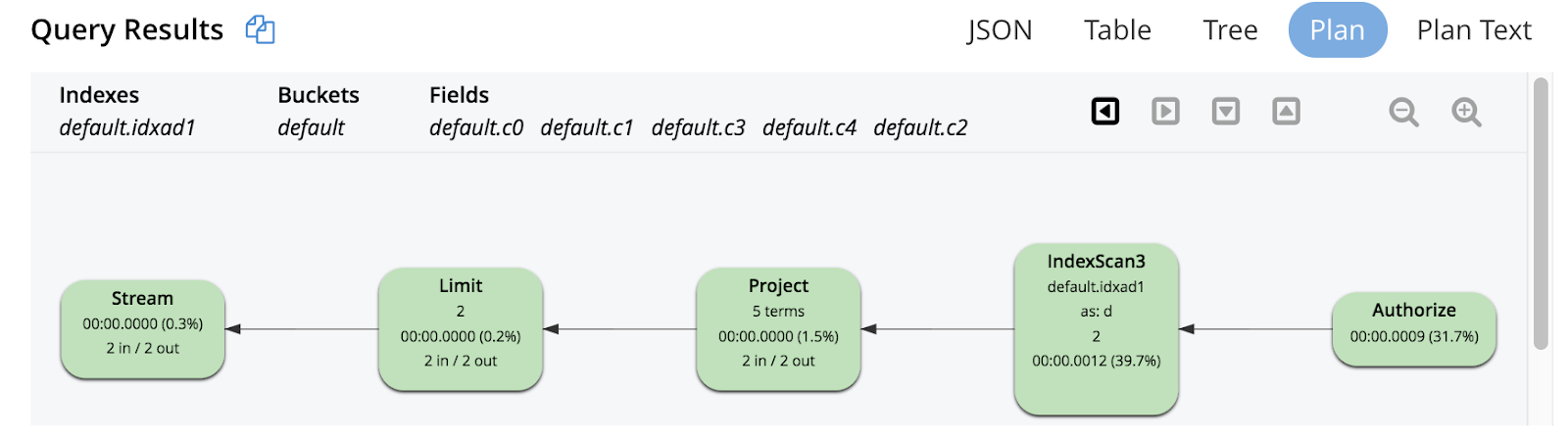
This example is similar to example 1 except it uses an array index. The above graphical execution tree shows index scan (IndexScan3) performing scan, index grouping aggregations, order, offset and limit. The results from the index scan are projected.

Example 5: Group and Aggregation of UNNEST Operation

Let's consider the following query and index:

SELECT v.id AS id, d.c0 AS c0, SUM(v.id) AS sumid, 
        AVG(d.c1) AS avgc1
FROM default AS d UNNEST d.a1 AS v 
WHERE v.id > 0 
GROUP BY v.id, d.c0;

Required index:

CREATE INDEX idxaa1 ON default(ALL ARRAY v.id FOR v IN a1 END, c0, c1);

The query has GROUP BY and multiple aggregates. The query has UNNEST on array d.a1 and has a predicate on the array key (v.id > 0). The index idxaa1 qualifies query (for UNNEST to use an array index for the index scan, the array index must be leading key and array variables in the index definition must match with the UNNEST alias). The predicate (v.id > 0) can be converted into exact range scans and passed to the index scan. Therefore, the index and query combination is suitable to handle index grouping and aggregations.

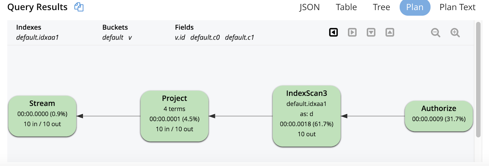
The above graphical execution tree shows index scan (IndexScan3) performing scan, index grouping aggregations. The results from the index scan are projected. The UNNEST is a special type of JOIN between parents and each array element. Therefore, UNNEST repeats the parent document fields (d.c0, d.c1) and the d.c0, dc.1 reference would have duplicates compared to the origina ld documents (you need to aware this while using in SUM() and AVG()).

Rules for Index Grouping and Aggregation

The index grouping and aggregation are per query block, and the decision on whether or not use index grouping/aggregation is made only after index selection process.

• Query block should not contain joins, NEST, or subqueries.
• Query block must be covered by a single line index.
• Query block should not contain ARRAY_AGG(). 
• Query block can't be correlated.
• All the predicates must be exactly translated into range scans.
• GROUP BY and aggregate expressions can't reference any subqueires, named parameters, or positional parameters.
• GROUP BY keys and aggregate expressions can be index keys, document keys, expressions on index keys, or expressions on document keys.
• An index needs to be able to do grouping and aggregation on all the aggregates in query block otherwise no index aggregation (i.e. all or none).
• Aggregate contains the DISTINCT modifier.
• The group keys must exactly match with leading index keys (if the query contains an equality predicate on the index key, then it assumes this index key is implicitly included in GROUP keys if not already present).
• The aggregate expression must be on one of the n+1 leading index keys (n represent the number of group keys).
• In case of partition indexes, the partition keys must exactly match with group keys.

Summary

When you analyze the explain plan, correlate the predicates in the explanation to the spans and make sure all the predicates exactly translated to range scans and queries are covered. Ensure queries use index grouping and aggregations, and if possible, query using full aggregations from the indexer by adjusting index keys for better performance.