A Trial Run With H2O AutoML in R: Automated Machine Learning Functionality

It has been a couple of years since we started catching on to automating machine learning and related activities. We had various discussions, theories, and ideas along those lines. But now, we are gradually beginning to witness advancements in ML automation techniques. The best part is that most auto ML packages are available for free. For example, TPOT is available as an open-source Python library for people to use. BigML recently announced Deepnets, the first deep learning service for non-experts. Similarly, H2O has released driverless AI and AutoML (referring to automated machine learning) — a significant relief for R users, as R didn't have any auto ML packages as Python had.

In this piece, we will walk through H2O's AutoML functionality and see what it does. 

Kickoff Modeling Excercise

Let's begin with loading the H2O library, initializing an H2O instance, and loading the data file. I will bypass and jump straight into H2O's AutoML functionality. 

library(h2o)
h2o.init()

conv_data <- read.csv("/conversion_data.csv")
str(conv_data)

There are six attributes in this data set. The objective of this modeling exercise is to improve the conversion rate of the users visiting the website. So, the prediction target attribute is converted and other attributes are going to be used as predictors.

Datatype Conversion

Dealing with categorical variables in machine learning is a significant task. They are sometimes the bottleneck in getting good results out of the model. The better we transform categorical variables, the more robust the results are. It is a science in itself and is a topic of discussion of its own. So, here, we stick to basic categorical data transformations.

conv_data$age <- as.factor(conv_data$age)  
conv_data$total_pages_visited <- as.factor(conv_data$total_pages_visited) 
conv_data$converted <- as.factor(conv_data$converted)  

# Country is a nominal attribute. When using the H2O algorithm, we can just convert it to factor so that it can be one hot encoded
#automatically
conv_data$country  <- as.factor(conv_data$country)  

conv_data$ID  <- 1:nrow(conv_data)  
conv_data.hex  <- as.h2o(conv_data)

Split Dataset

It is essential to ensure that the model we built works well on the new datasets when deployed in a real production environment. So, the data used for modeling is divided into multiple sets, typically in a ratio of 60:20:20. The largest split is used for training the model, and one of the other two divisions is passed on to the modeling function as a validation set that is used by the algorithm to validate/tune the model. The last one is used as a test set (considered to be a dummy production environment), which is used independently to test the predictions and evaluate the accuracy of the model.

#Split data into Train/Validation/Test Sets

split_h2o <- h2o.splitFrame(conv_data.hex, c(0.6, 0.2), seed = 1234 )

train_conv_h2o <- h2o.assign(split_h2o[[1]], "train" ) # 60%
valid_conv_h2o <- h2o.assign(split_h2o[[2]], "valid" ) # 20%
test_conv_h2o  <- h2o.assign(split_h2o[[3]], "test" )  # 20%

#Model

# Set names for h2o
target <- "converted"
predictors <- setdiff(names(train_conv_h2o), target)

AutoML

After all these basic preprocessings, now is the time to create models. We run h2o.automl() by setting few mandatory parameters as below. 

• x: The names of the predictors

• y:  The target column name

• training_frame: The training data set that is to be used for creating the model

• leaderboard_frame: The validation data set used by h2o to ensure the model doesn't overfit the data

You can follow the H2O AutoML documentation for more information on the AutoML functionality and parameters

# Run the automated machine learning 
automl_h2o_models <- h2o.automl(
    x = predictors, 
    y = target,
    training_frame    = train_conv_h2o,
    leaderboard_frame = valid_conv_h2o
    )

Leader

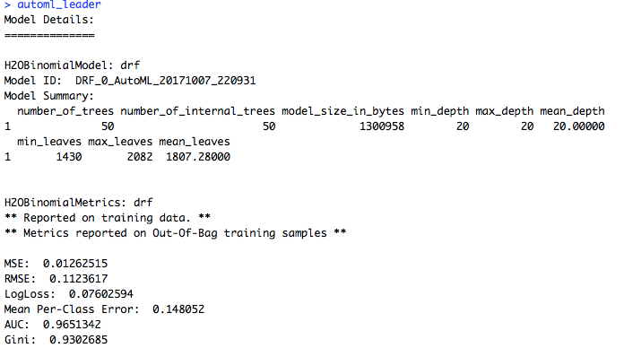
All of the models are stored the automl_h2o_models object. However, we are only concerned with the leader, which is the best model in terms of accuracy on the validation set. We’ll extract it from the models object.

# Extract leader model
automl_leader <- automl_h2o_models@leader

The best model for this exercise given out by AutoML is a DRF (distributed random forest) model with a 96.5% AUC.

Prediction

Now, let's use the model to predict the conversion of the test data. As the holdout test set is not used in creating the model, this is a real test of performance that we might see in a live production environment.

# Predict on hold-out test set
pred_conversion <- h2o.predict(object = automl_leader, newdata = test_conv_h2o)
#Confusion matrix on test data set
h2o.table(pred_conversion$predict, test_conv_h2o$converted)

The prediction accuracy is around 98.5%, recall is 71.2%, and precision is 80%. These are pretty decent figures and can be considered as a reliable production-ready model.

Performance

You can also use h2o.performance()  to evaluate a model. The result has all the performance measures that can be computed for that model. You can even use this result object to derive other evaluation metrics such as confusion matrix, accuracy, tpr, fpr, F1, etc. Track and choose the best metrics you want to evaluate your model. 

#compute performance
perf <- h2o.performance(automl_leader,conv_data.hex)
h2o.confusionMatrix(perf)
h2o.accuracy(perf)
h2o.tpr(perf)

For me, AutoML is a neat feature that can save a lot of time! No more coding for different models, noting down the results, and selecting the best model. AutoML is going to do all of these for you while you brew a cuppa!