Beyond Reactive HPA: Designing a Predictive Autoscaler with KEDA and Time-Series Forecasting

Kubernetes scaling relies predominantly on the Horizontal Pod Autoscaler (HPA), a robust feedback loop that adjusts capacity based on observed metric saturation. While reliable for steady-state traffic, HPA is inherently reactive, it mitigates resource exhaustion only after it has begun.

For workloads with steep, predictable traffic ramps (such as morning log-in spikes or scheduled synchronization jobs), this reactive lag guarantees a period of transient performance degradation. To achieve strict Service Level Objectives (SLOs) during these ramps, infrastructure must shift from reacting to current load to anticipating future demand. This article details a feed-forward architecture using time-series forecasting (Prophet) and Kubernetes Event-Driven Autoscaling (KEDA) to provision capacity before the demand arrives.

The Structural Limitation of Reactive HPA

The Horizontal Pod Autoscaler operates as a feedback controller. It samples a metric at fixed intervals, compares it against a target value, computes a desired replica count, and applies scaling adjustments conservatively to avoid oscillation.

This design is intentional. HPA trades responsiveness for stability. It smooths replica changes using stabilization windows and scale-up/down policies to prevent flapping. In steady workloads, this behavior is desirable.

The weakness lies in timing. Consider a realistic morning ramp scenario:

CPU crosses 75% at 09:00:20
HPA reconciliation triggers at 09:00:30
Pod scheduled at 09:00:40
Container starts at 09:01:05
Readiness passes at 09:01:25

Effective capacity increases roughly 60-90 seconds after saturation begins.

That 60-90 seconds is not a configuration error. It is the accumulated latency of:

• Metrics collection interval
• HPA reconciliation interval
• Scheduler queue delay
• Image pull (if not cached)
• Container initialization
• Readiness probe stabilization
• Application warm-up (JIT, connection pools, cache fill)

During that window:

• Tail latency increases
• Connection pools saturate
• Retry traffic amplifies pressure
• Error budgets are consumed

Reactive scaling corrects the system eventually, but it absorbs avoidable performance degradation. For unpredictable bursts, this is acceptable. For predictable daily ramps, it is unnecessary.

If traffic ramps at roughly the same time every weekday, the system is repeatedly absorbing known, forecastable stress.

Control Model: Adding Feed-Forward Scaling

Reactive scaling reduces error after it appears. Predictive scaling introduces a feed-forward component that anticipates load based on historical patterns.

Conceptually:

Where "ScaleLatency" equals the measured end-to-end time from the metric trigger to pod readiness. You should instrument:

• Time from scaling decision --> pod scheduled
• Time from scheduled --> container running
• Time from running --> readiness
• Time from readiness --> latency normalization

To gain a performance advantage, your forecasting window must exceed the 90 second scaling delay, predicting only 30 seconds out leaves you unequipped to handle the surge.

The predictive signal does not replace reactive control. It complements it, reducing transient error while preserving stability. This hybrid structure is critical. Predictive-only scaling would be fragile. Reactive-only scaling remains slow for known ramps. Together, they form a more stable control system.

Architecture Overview

The architecture introduces a forecasting service that continuously predicts near-future workload and publishes that prediction as a metric consumed by Kubernetes.

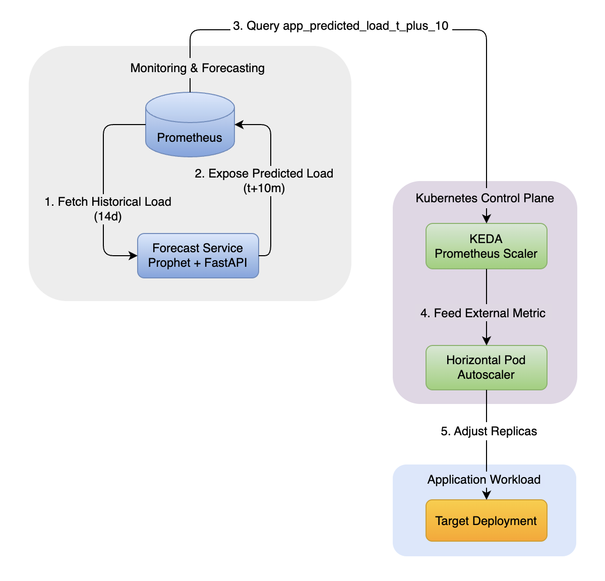
Prometheus stores historical request rates. The forecast service consumes that history, predicts future load, and exposes it. KEDA queries Prometheus for this prediction and feeds it into HPA. Kubernetes scaling remains intact. We are enriching its inputs, not replacing its control path.

This design deliberately avoids:

• Custom Kubernetes controllers
• Scheduler plugins
• Forking HPA
• Direct manipulation of replica sets

We treat predicted demand as just another metric. That keeps:

• Observability intact
• Debuggability simple
• Failure domains isolated

If the forecast service crashes, HPA continues operating reactively. The cluster does not depend on prediction for survival.

Forecasting Service Implementation

Before scaling decisions can incorporate predictive signals, the system must convert historical workload into a short-horizon forecast.

The forecasting service has two distinct responsibilities:

1. Model training (expensive, periodic)
2. Inference (fast, continuous)

Training involves:

• Fetching historical time-series data
• Cleaning and transforming it
• Fitting seasonality-aware models
• Storing the trained model in memory

Inference must:

• Be constant-time
• Avoid blocking
• Never trigger retraining

The forecast horizon must exceed measured scale latency. A five to ten minute horizon typically covers daily ramp scenarios and allows sufficient reaction time.

Below is the production-grade implementation using FastAPI and BackgroundScheduler:

import logging
from fastapi import FastAPI
from prometheus_api_client import PrometheusConnect
from prophet import Prophet
import pandas as pd
from datetime import datetime, timedelta
from apscheduler.schedulers.background import BackgroundScheduler

# Configuration
PROMETHEUS_URL = "http://prometheus-service.monitoring.svc.cluster.local:9090"
METRIC_QUERY = 'sum(rate(http_requests_total[5m]))'
FORECAST_WINDOW_MINUTES = 10

app = FastAPI()
prom = PrometheusConnect(url=PROMETHEUS_URL, disable_ssl=True)
model_cache = {"model": None, "last_trained": None}

def train_model():
    """
    Heavy Job: Fetches 14 days of data and fits the Prophet model.
    Scheduled to run once every hour to avoid blocking the API.
    """
    logging.info("Starting model training...")
    try:
        data = prom.get_metric_range_data(
            metric_name=METRIC_QUERY,
            start_time=(datetime.now() - timedelta(days=14)),
            end_time=datetime.now()
        )
        
        df = pd.DataFrame(data[0]['values'], columns=['ds', 'y'])
        df['ds'] = pd.to_datetime(df['ds'], unit='s')
        df['y'] = pd.to_numeric(df['y'])

        m = Prophet(daily_seasonality=True, weekly_seasonality=True)
        m.fit(df)
        
        model_cache["model"] = m
        model_cache["last_trained"] = datetime.now()
        logging.info("Model training complete.")
    except Exception as e:
        logging.error(f"Training failed: {e}")

scheduler = BackgroundScheduler()
scheduler.add_job(train_model, 'interval', minutes=60)
scheduler.start()

train_model()

Operational considerations:

• Persist the trained model to disk or object storage for restart resilience.
• Expose model_last_trained_timestamp as a Prometheus metric.
• Alert if retraining fails repeatedly.
• Cap historical window size to prevent memory growth.

Prediction quality is less important than directional correctness. The goal is not perfect forecasting. The goal is early capacity allocation.

Exposing the Predictive Metric

The forecast service must expose predicted load in a format consumable by Kubernetes. Instead of a custom JSON adapter, we utilize the standard Prometheus Exposition Format. This allows KEDA to use its native Prometheus scaler, which is significantly more robust than the generic External scaler.

This keeps integration simple:

• No custom metrics adapters
• No Kubernetes API extensions
• No side-channel communication

@app.get("/metrics")
def get_metrics():
    """
    Exposes the PREDICTED load for KEDA to scrape.
    """
    if not model_cache["model"]:
        return "# HELP model_loading Model is still training\n# TYPE model_loading gauge\nmodel_loading 1"

    future_df = model_cache["model"].make_future_dataframe(periods=FORECAST_WINDOW_MINUTES, freq='min')
    forecast = model_cache["model"].predict(future_df)
    
    predicted_val = forecast.iloc[-1]['yhat']
    predicted_val = max(0, predicted_val)

    return f"""# HELP app_predicted_load_t_plus_10 Predicted requests per second 10m from now
# TYPE app_predicted_load_t_plus_10 gauge
app_predicted_load_t_plus_10 {predicted_val}
"""

The service must degrade gracefully. If forecasting fails, the metric endpoint should return the last known good value or an error code that prevents KEDA from scaling to zero.

Inference must remain lightweight. Prometheus scrapes this endpoint at fixed intervals. If inference exceeds scrape timeout, scaling responsiveness degrades.

Clamp outputs:

• No negative predictions
• Optional upper bound protection
• Avoid NaN values

Prediction is advisory, not authoritative.

Integrating with KEDA

KEDA allows external metrics to influence HPA without modifying Kubernetes core components. We configure KEDA to query the predicted metric (app_predicted_load_t_plus_10) rather than the current load.

A representative ScaledObject configuration:

apiVersion: keda.sh/v1alpha1
kind: ScaledObject
metadata:
  name: predictive-scaler
spec:
  scaleTargetRef:
    name: my-service
  minReplicaCount: 2
  maxReplicaCount: 50
  pollingInterval: 15
  triggers:
  - type: prometheus
    metadata:
      serverAddress: http://prometheus-service.monitoring.svc.cluster.local:9090
      metricName: app_predicted_load_t_plus_10
      query: app_predicted_load_t_plus_10
      threshold: '100'

The threshold must be calibrated using load testing.

If one pod handles 120 RPS at 70% CPU, setting threshold to 100 creates headroom. Do not guess this value. Reactive CPU-based HPA should remain active. Predictive scaling augments, not replaces, feedback control.

Defense: Why Not Just Use Cron?

A frequent counter-argument is the simplicity of Cron-based scaling (e.g., "Scale to 50 replicas at 08:55 AM"). While Cron is simpler to implement, it is brittle in operation.

If the forecast underestimates demand, reactive scaling compensates. If it overestimates demand, cluster-level limits constrain cost exposure.

This max-selection strategy ensures predictive scaling improves latency without becoming a single point of failure.

Failure Modes and Guardrails

Predictive systems introduce distinct risks. Over-prediction increases infrastructure cost. To control this, predictive replicas should be capped relative to observed reactive demand.

Persistent divergence between predicted and actual load should trigger automatic decay of predictive influence.

Under-prediction is mitigated by reactive scaling but should trigger recalibration if sustained.

Concept drift must be detected through rolling mean absolute error (MEA) and variance monitoring. Forecast error should itself be exported as a Prometheus metric.

When drift exceeds defined thresholds, predictive scaling should disable itself automatically. The forecast service must be isolated from core scaling control paths to avoid cascading failure.

Predictive autoscaling must fail safe. If the forecasting path collapses, reactive HPA continues functioning normally.

Quantified Benefit

Consider a ramp from 200 RPS to 1000 RPS over five minutes.

Reactive-only systems exhibit 60-90 seconds of elevated tail latency as scaling catches up incrementally.

Hybrid systems provision capacity before saturation, reducing transient error and oscillation amplitude.

The improvement is most visible in p95 and p99 latency rather than average latency. Average latency may appear similar. Tail behavior improves materially.

In latency-sensitive systems, that distinction determines SLO compliance.

Closing Perspective

Reactive autoscaling mitigates stress after it appears. Predictive autoscaling reduces stress before it materializes.

By combining feed-forward forecasting with feedback stabilization, Kubernetes scaling shifts from reactive correction toward anticipatory control. In environments with predictable load ramps and strict latency objectives, this approach eliminates a class of avoidable performance degradation without replacing proven control mechanisms.

The architecture remains operationally conservative:

• Reactive control remains primary safety.
• Prediction augments, not dictates.
• Failure degrades gracefully.

That balance is what makes predictive autoscaling practical rather than experimental.