How Go Maps Work: From Buckets to Swiss Tables

Hey Mates!

“How does a map work in Go?” is one of my favorite interview questions. It sounds simple, but it opens up a conversation about hashing, collisions, memory layout, and why two implementations with the same average O(1) lookup complexity can behave quite differently. With Go 1.24, that conversation got more interesting: the map implementation switched to Swiss Tables. Let’s walk through how the old implementation worked, what changed, and how the new design finds your keys.

TL;DR

Go 1.24, released in February 2025, completely replaced the internal implementation of the built-in `map` with a design based on Google's Swiss Tables. The syntax and the behavior guaranteed by the Go specification did not change, so existing programs required no migration. In microbenchmarks, some map operations became up to 60% faster. Across the Go team's full-application benchmark suite, geometric mean CPU time improved by about 1.5%. Datadog reported roughly 70% less memory for one exceptionally large map—an impressive case study, not a universal promise.

Why Replace map at All?

map is one of the most frequently used data structures in Go. It appears in caches, configuration, indexes, and every `map[string]any` we would rather not discuss. The old implementation served Go well for more than a decade.

Hash-table research did not stop, however. At CppCon 2017, Google engineers Sam Benzaquen, Alkis Evlogimenos, Matt Kulukundis, and Roman Perepelitsa presented a new cache-friendly design. It became known as Swiss Tables, after the Google Zürich office where the team worked. In 2018, Google released an implementation in the C++ Abseil library. The design then spread across ecosystems:

• C++: absl::flat_hash_map in Abseil;
• Rust: the standard HashMap is built on hashbrown, a Swiss Tables implementation, since Rust 1.36;
• Go: first through third-party packages such as dolthub/swiss and cockroachdb/swiss, then in the built-in map starting with Go 1.24.

The route into Go was collaborative. Community members built early prototypes. Peter Mattis of CockroachDB combined those ideas with solutions for Go-specific requirements in cockroachdb/swiss. The Go 1.24 runtime implementation is heavily based on that work.

Before we get to the “Swiss” part, let us quickly review hash tables. If collisions and load factors are already familiar, skip to section 3.

Hash Tables From First Principles

Imagine a theater coat check where coats are retrieved by surname. You say “Smith,” and the attendant applies a simple rule to decide which section to search first, section 17, perhaps. They do not scan the entire room; they go directly to one small area and inspect a few tags.

• The key is the surname.
• The value is the coat.
• The hashfunction turns a key into the starting section. The same key always produces the same result within a particular map.
• A slot stores one key/value pair.

Lookup is O(1) on average because the hash takes us to a small part of the table instead of forcing us to scan every entry. This is an average-case property, not an unconditional guarantee.

The unavoidable problem is a collision: there are finitely many locations, so different keys eventually choose the same starting point. Two classic strategies handle this:

1. Chaining. Section 17 holds a list of key/value pairs. Lookup walks that small list. Hans Peter Luhn of IBM described this approach in 1953.
2. Open addressing. Slot 17 is occupied, so try another slot, then another, until a suitable one is found. The order of locations is called the probe sequence. Open addressing was used in 1954 and formally published in 1957.

Both ideas are about 70 years old. The interesting part is how modern implementations make them friendly to modern CPUs.

The Old Implementation: Go 1.23 and Earlier

The old Go map was a hybrid. It used fixed-size buckets, while excess collisions were handled with chains of overflow buckets. In spirit, it was closer to chaining.

A map had an hmap header pointing to an array of buckets. Each `bmap` bucket contained exactly 8 slots:

flowchart LR
    subgraph HMAP["hmap header"]
        direction TB
        C["count: number of entries"]
        B["B: log2 bucket count"]
        P["buckets: array pointer"]
    end
    P --> ARR["bucket array: 2^B buckets"]
    ARR --> BKT
    subgraph BKT["bmap bucket: 8 slots"]
        direction TB
        TH["tophash: 8 filter bytes"]
        K["8 keys"]
        V["8 values"]
        OV["overflow pointer"]
    end
    OV --> OB1["overflow bucket"]
    OB1 --> OB2["another overflow bucket"]

Three details matter:

• tophash: Eight bytes at the start of the bucket, one per slot. Each byte contains the top bits of that key's hash. Comparing a byte is cheaper than comparing a full string key, so it acts as a fast filter.
• Keys and values are stored separately: Eight keys followed by eight values. This reduces alignment padding.
• Overflow buckets: When the primary bucket cannot hold another entry, the runtime allocates another bucket and links it into a chain.

To find grape, the runtime roughly did this:

1. Calculate `hash("grape")`.
2. Use the low `B` bits to select a bucket.
3. Check the bucket's eight `tophash` bytes one at a time.
4. When a byte matches, compare the full key. If the key matches, return the value.
5. If the bucket has no match, follow its pointer to the overflow bucket and repeat.
6. If the chain ends, the key is absent.

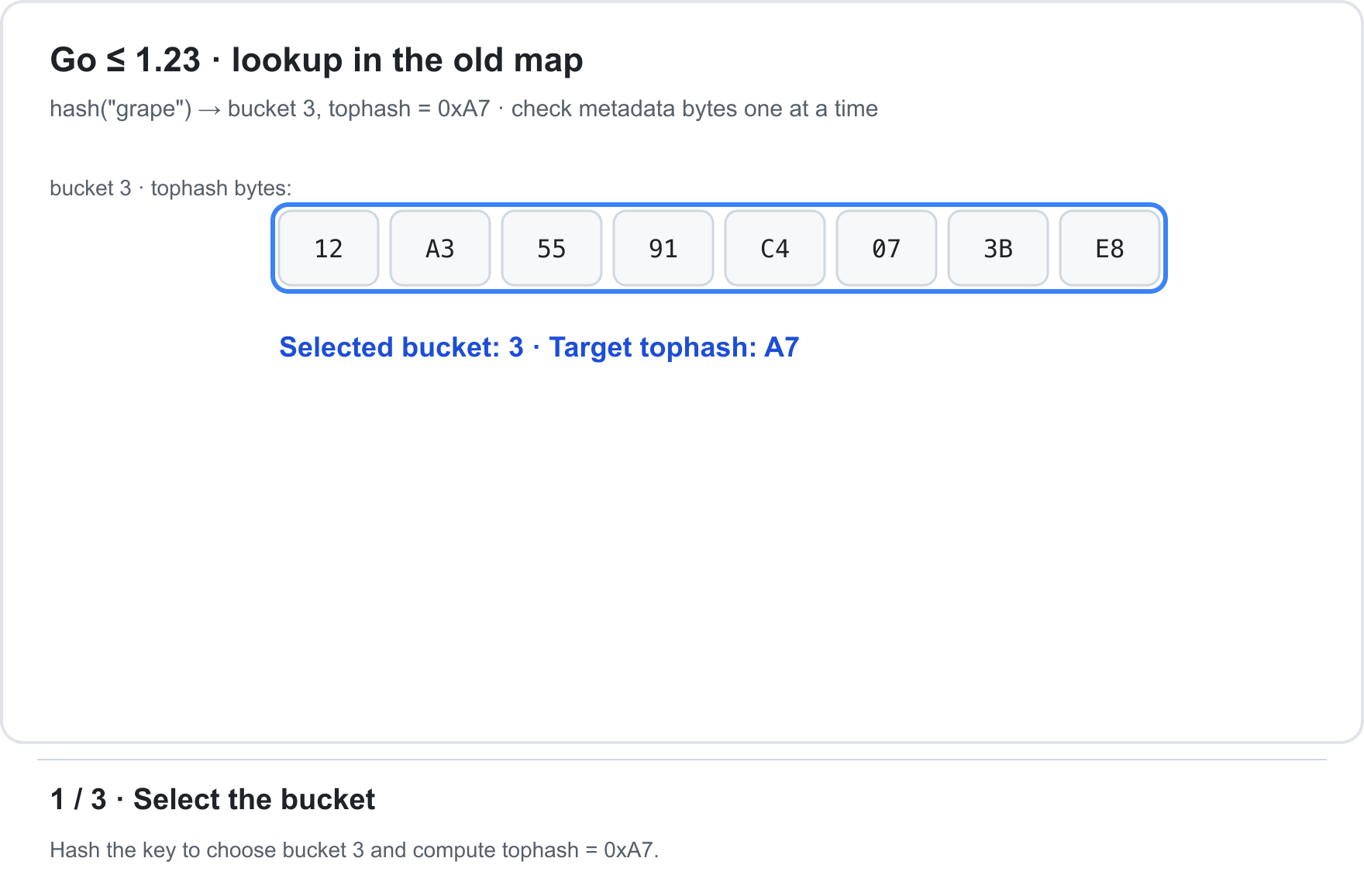
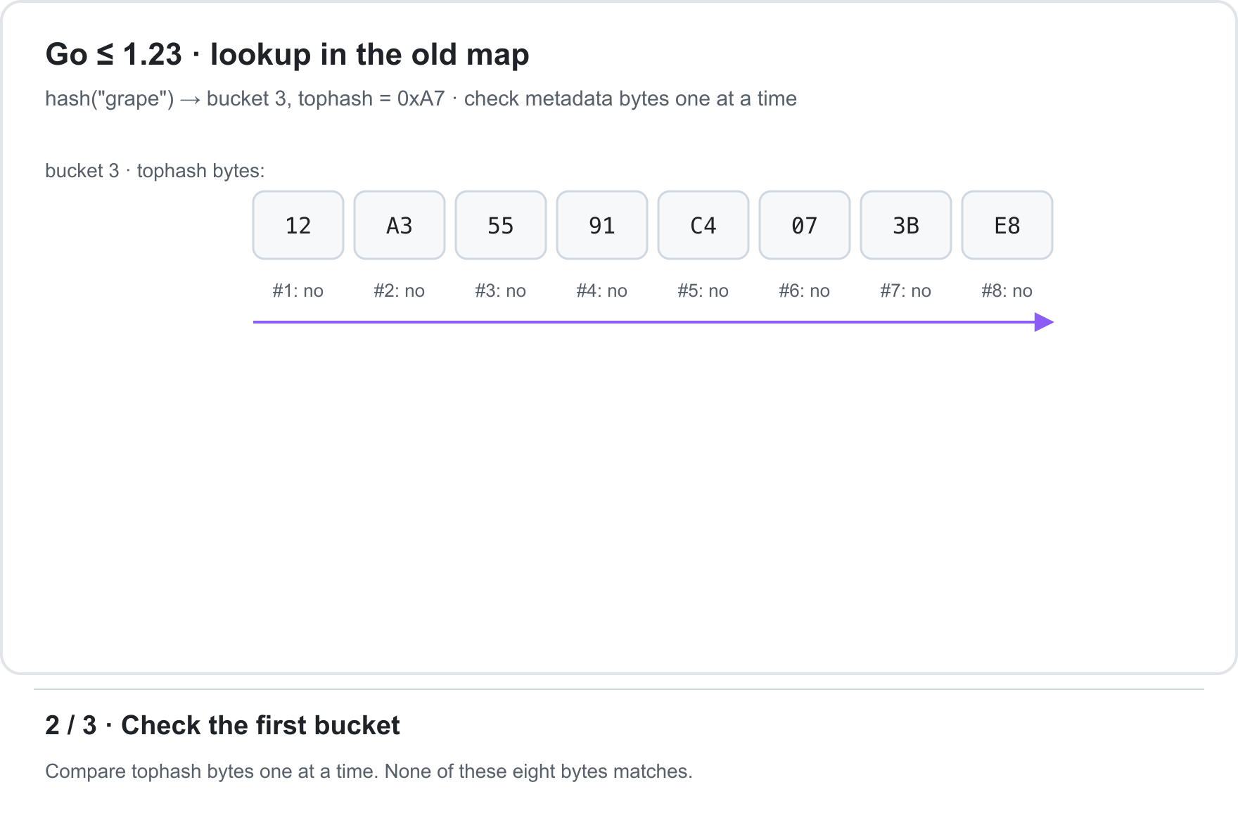
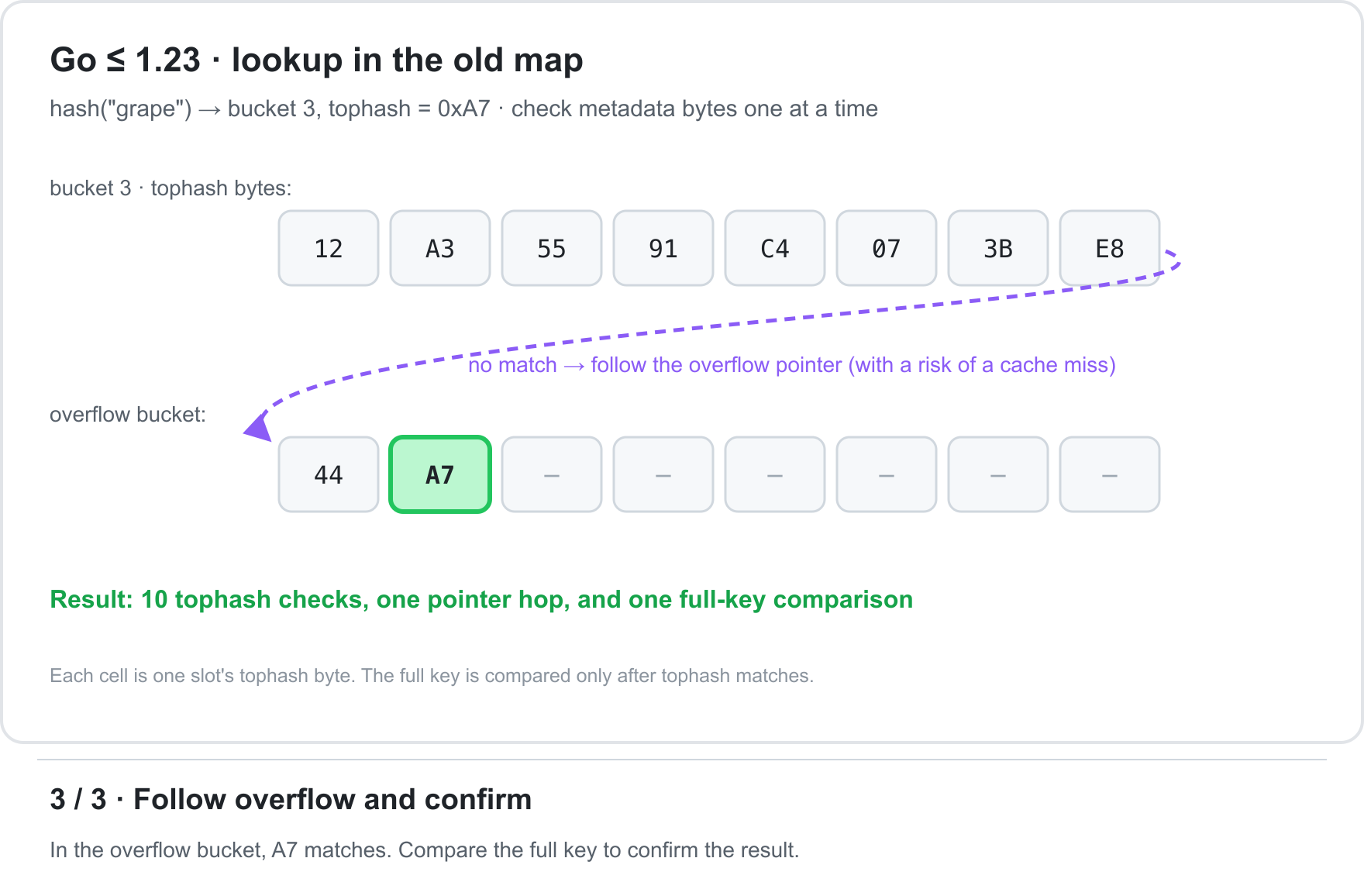
The old map grew when average occupancy exceeded 6.5 entries per 8-slot bucket, a load factor of 81.25%, or when too many overflow buckets accumulated. The number of primary buckets doubled.

Crucially, growth was incremental. Go did not move the entire old array at once. Each write evacuated a little more data. One unlucky insertion therefore did not have to copy a gigabyte-sized map in a single pause.

• Pointer chasing. Every overflow hop reads another part of the heap and increases the risk of a CPU-cache miss. A long overflow chain can therefore be expensive.
• Serial metadata checks. The runtime inspected `tophash` byte by byte and slot by slot. Eight slots could mean eight loop iterations and several branches.
• Memory overhead. Overflow buckets and their pointers cost memory. Raising the load factor much above 81% made overflow chains more common and lookup slower. The garbage collector could also have more pointers to scan.

The goal was clear: fewer pointers, better locality, and less serial work. Swiss Tables provide exactly that.

Meet Swiss Tables

A Swiss Table is open addressing adapted to modern CPUs. Three decisions drive the design:

1. Split the hash into an address and a short fingerprint.
2. Pack the metadata for a group of slots into one machine word.
3. Compare the fingerprints of 8 slots in parallel, then compare full keys only for the candidates.

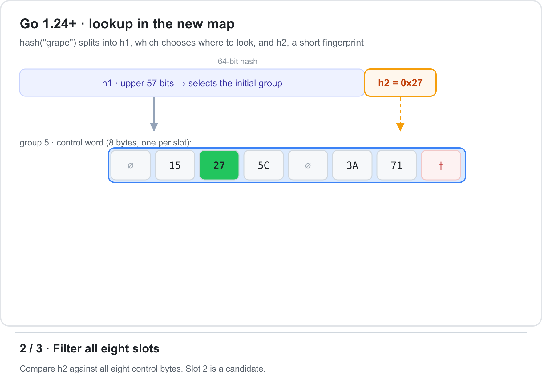
A 64-bit hash is divided into two unequal pieces:

                       64-bit key hash
┌─────────────────────────────────────────────┬─────────────┐
│              h1: upper 57 bits              │ h2: 7 bits  │
│       chooses where probing begins          │ fingerprint │
└─────────────────────────────────────────────┴─────────────┘

• h1 selects the initial group.
• h2 is a 7-bit fingerprint used as a cheap filter before a full-key comparison.

In the coat-check analogy, h1 chooses a section, and h2 is a short mark on each tag that quickly rules out unrelated coats.

Slots are arranged in groups of 8. Each group has a 64-bit control word, one byte per slot:

control word: 64 bits = 8 bytes

  ┌────┬────┬────┬────┬────┬────┬────┬────┐
  │ ∅  │ 15 │ 27 │ 5C │ ∅  │ 3A │ 71 │ †  │
  └────┴────┴────┴────┴────┴────┴────┴────┘
     │    │                             │
     │    └─ occupied, h2 = 0x15        └─ deleted tombstone
     └─ empty

Each byte describes its slot:

| Byte value             | Meaning |
| `0b1000_0000` (`0x80`) | **empty** slot |
| `0b1111_1110` (`0xFE`) | **deleted** slot, or tombstone |
| `0b0xxx_xxxx`          | occupied; the low seven bits contain h2 |

Occupied slots always have a zero high bit, while empty and deleted slots have a one. That encoding enables efficient parallel tests.

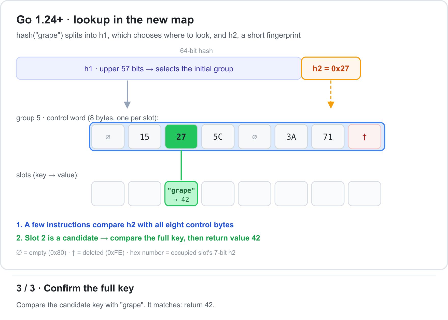
Suppose we are looking for h2 = 0x27. Conceptually, the operation looks like this:

probe word:   27 │ 27 │ 27 │ 27 │ 27 │ 27 │ 27 │ 27
              == │ == │ == │ == │ == │ == │ == │ ==
control word:  ∅ │ 15 │ 27 │ 5C │  ∅ │ 3A │ 71 │  †
result:        0 │  0 │  1 │  0 │  0 │  0 │  0 │  0
                       ↑
                  candidate slot 2

On amd64, Go recognizes this operation as an intrinsic and uses SIMD instructions. Other architectures have a portable SWAR implementation — SIMD Within A Register — that processes all eight bytes using arithmetic on one 64-bit word.

The following simplified code is optional. The important result is a bit mask of slots whose h2 may match:

func matchH2(ctrl uint64, h2 uint8) uint64 {
    broadcast := uint64(h2) * 0x0101010101010101
    x := ctrl ^ broadcast
    return (x - 0x0101010101010101) &^ x & 0x8080808080808080
}

There are two reasons a candidate is not yet a result:

1. h2 has only seven bits, so an occupied slot has a 1/128 chance of sharing the same fingerprint by accident;
2. The portable bit trick can produce a rare extra candidate because of subtraction borrow.

Neither affects correctness. Go always performs a full-key comparison before returning a value.

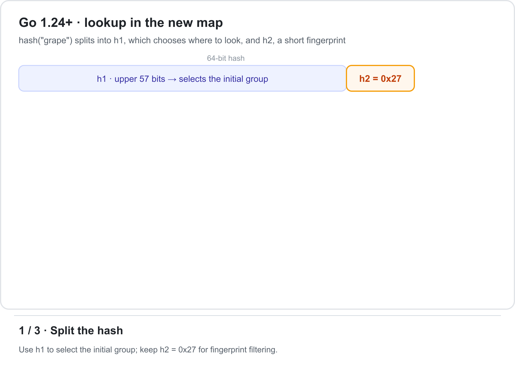
If the initial group has no matching key, open addressing continues at group granularity. Go uses a quadratic probe sequence. Three rules are enough to understand lookup:

• Matching h2 bytes produce candidate slots whose full keys are checked;
• If the group contains an empty slot, stop — the key is absent;
• If the group has no match and no empty slot, visit the next group in the probe sequence.

One probe handles the metadata for eight slots, so densely populated tables can still be searched efficiently.

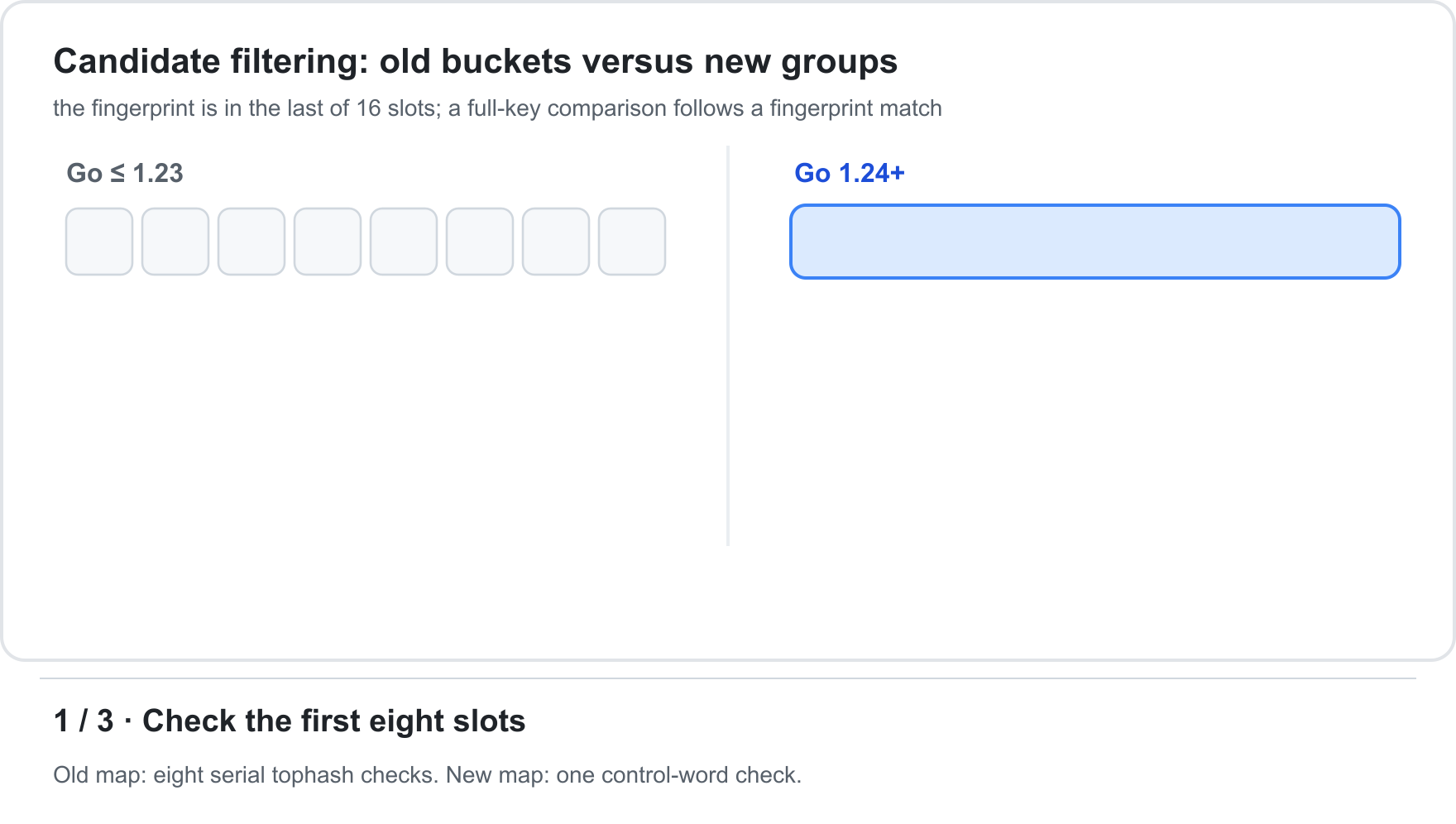
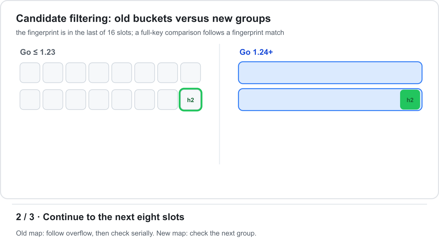
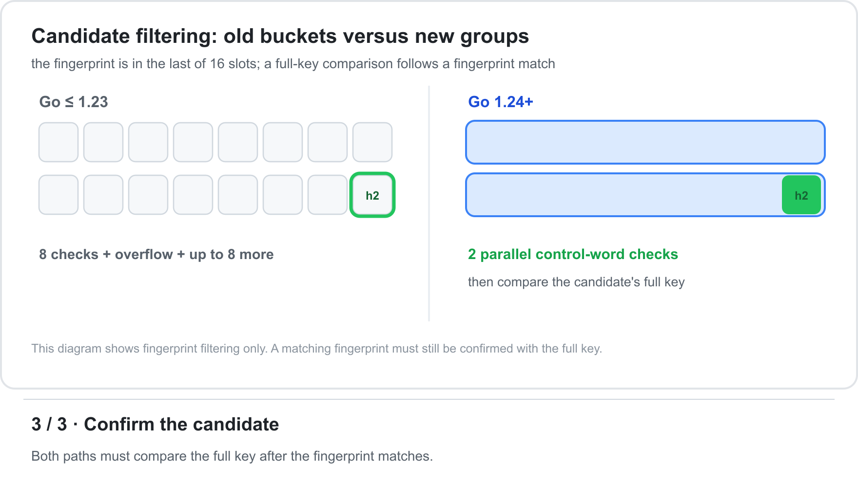
Because group metadata is cheaper to inspect, Swiss Tables can remain more densely populated. Go allows an average load up to 7/8 = 87.5%, compared with 81.25% in the old implementation. More useful entries in the same backing storage usually means less memory per key.

Go's Extension: A Directory of Tables

Go could not simply port Abseil's implementation. Two language and runtime requirements needed additional design work.

A conventional Swiss Table grows all at once: allocate a larger array and move every entry. For a gigabyte-sized map, the insertion that triggers growth would suffer a noticeable pause. Go is widely used for latency-sensitive services, and its old maps already bounded growth work per insertion.

A large Go map is a directory of independent Swiss Tables, not one unbounded table. Each table covers part of the hash space and has a maximum capacity of 1024 slots, or 128 groups:

flowchart TD
    M["map[K]V"] --> DIR["directory: array of table pointers"]
    DIR --> T0["table 0: up to 1024 slots"]
    DIR --> T1["table 1: up to 1024 slots"]
    DIR --> TN["table N"]
    T1 --> G0["group 0: control word + 8 slots"]
    T1 --> G1["group 1: control word + 8 slots"]
    T1 --> GK["up to 128 groups"]

A variable number of upper hash bits selects the table. This technique is a form of extendible hashing.

Growth is local. When a table below the limit fills, only that table grows. Once a table reaches the limit, it splits into two. The amount of growth work caused by one insertion is therefore bounded by one table of at most 1024 slots: roughly at most 896 live entries at the 7/8 load threshold (not the entire map).

Small maps get a special fast path. A map that starts small and never exceeds 8 entries lives directly in a single group with no table directory. A map that has already grown, or was created with a large `hint`, does not shrink back into this representation after deletions.

Unlike many hash tables, Go explicitly permits modifying a map during iteration:

1. an entry deleted before it is reached must not be produced;
2. an entry updated before it is reached must produce its latest value;
3. a newly inserted entry may or may not be produced.

Growth reshuffles storage, so an iterator cannot simply walk the current array. Go's iterator retains the old table to determine traversal order. Before returning an entry, it consults the current table to confirm that the key still exists and to obtain the latest value. According to the Go team, iteration is the most complex part of the implementation.

Deletion and Tombstones

With open addressing, deleting an entry cannot always turn its slot into an ordinary empty slot. Lookup stops at an empty slot. Creating one in the middle of another key's probe sequence could therefore make a live key unreachable.

A tombstone, encoded as deleted (`0xFE`), means: “an entry used to be here; continue probing.” Insertions may reuse tombstones.

Go avoids a tombstone when the group already contains another empty slot. Any lookup reaching that group would stop there anyway, so turning the deleted slot into empty cannot break a probe sequence.

Accumulated tombstones disappear during a later grow or split. Live entries are copied into new groups and deleted slots are not. Go 1.24 does not implement a separate same-size grow for this purpose.

And Performance Numbers

According to the Go team and early production reports:

1. Microbenchmarks: some map operations are up to 60% faster than in Go 1.23. Results vary widely, and a few edge cases regress.
2. Full-application benchmarks: the Go team's suite showed about 1.5% geometric-mean CPU-time improvement for the whole application. A specific program may behave differently.
3. Memory: Datadog measured roughly 70% less map memory for one very large map with about 3.5 million entries in a high-traffic environment. This favorable case benefited from denser storage, no overflow buckets, and growth that did not retain two enormous bucket arrays at once. Savings were much smaller in another environment.

Large maps often benefit more because overflow chains and cache misses hurt the old design more strongly. The exact result depends on key and value sizes and on the mix of reads, writes, deletes, hits, and misses. Measure your own workload.

Takeaways

The Go Swiss Tables story is a good example of changing a foundational component carefully:

1. Start with a proven design already used by Abseil and Rust's `hashbrown`.
2. Adapt it to Go's invariants: bounded growth latency and modification during iteration.
3. Preserve the public API and specified behavior.

Hash tables are seven decades old, yet a better match between data layout and modern hardware can still remove CPU time and memory across a large ecosystem. “Solved” problems often have room for another good engineering pass.

References

• [Faster Go maps with Swiss Tables] — the primary Go team article
• [Go 1.24 Release Notes] — runtime changes and `GOEXPERIMENT=noswissmap`
• [Go 1.24 `internal/runtime/maps` source] — original source
• [Go 1.26 runtime source] — the release in which the old map implementation was removed
• [Abseil Swiss Tables Design Notes] — original source
• Matt Kulukundis at CppCon 2017
• Datadog's workload-specific memory case study
• [`hashbrown`] — the Swiss Tables implementation behind Rust's standard `HashMap`