A Fresh Look at Optimizing Apache Spark Programs

I have spent countless hours debugging slow Spark jobs, and it almost always comes down to a handful of common pitfalls. Apache Spark is a powerful distributed processing engine, but getting top performance requires more than just running your code on a cluster. Even with Spark’s built-in Catalyst optimizer and Tungsten execution engine, a poorly written or configured Spark job can run slowly or inefficiently. 

In my years as a software engineer, I have learned that getting top performance from Spark requires moving beyond the defaults and treating performance tuning as a core part of the development process. In this article, I will share the practical lessons I use to optimize Spark programs for speed and resource efficiency.

Overview: The goal is to tackle performance from every angle. We will start at the top with cluster-level configurations like resource allocation and memory, then dive right into the code to cover best practices for writing efficient Spark APIs. From there, we will get into the often overlooked but critical layer of data storage and formatting for faster I/O. To wrap it all up, we will see how monitoring the Spark UI and logs is key to refining performance over time. 

Prelude: Understanding Spark’s Architecture and Lazy Evaluation

Before we get into performance optimization, it helps to anchor on how Spark runs your program.

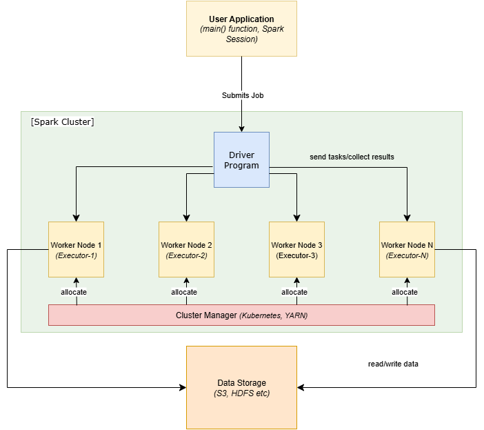
Driver: The driver program runs your main Spark application, builds a logical plan (a DAG of transformations), turns it into a physical plan, and schedules tasks across the Executor programs. It tracks job progress and collects results.

Executors: Executors live on worker nodes. They run tasks in parallel, keep partitions of data in memory or on disk, and spill to disk if needed. Executors are where your transformations actually execute.

Cluster Manager (allocator): YARN, Kubernetes, or Spark’s standalone manager decides how many executors you get and where they run. With the right settings, Spark can scale executors up/down as workload changes.

Lazy evaluation: Transformations like select, filter, groupBy, and join do not execute immediately. Spark builds a plan and only materializes work when you call an action (count, collect, write, show, etc.). This gives Spark the chance to:

• Push filters down to the data source
• Prune unused columns
• Reorder operations
• Choose efficient join/partition strategies

Spark Configuration Tuning

Spark offers many knobs and configuration properties that can significantly impact performance. Proper tuning of these settings ensures that your Spark cluster resources are used optimally. Key areas include dynamic resource allocation, memory management, and setting the right level of parallelism for shuffles.

1. Dynamic Resource Allocation

By default, Spark uses a static number of executors for the entire application. However, in real-world scenarios, data sizes can vary from one job run to another or even between stages of a single job. Allocating a fixed number of executors can either waste resources or cause bottlenecks. Dynamic Resource Allocation allows Spark to scale the number of executors up or down based on workload. This means Spark can add executors when your job has a lot of work and removes them when they are no longer needed, improving efficiency.

To enable dynamic allocation, set spark.dynamicAllocation.enabled to true in your Spark configuration. You should also ensure the cluster is configured to support this by enabling either the external shuffle service or Spark’s internal shuffle tracking (via spark.shuffle.service.enabled or spark.dynamicAllocation.shuffleTracking.enabled). Additionally, you can tune related settings such as the minimum and maximum number of executors Spark can allocate (spark.dynamicAllocation.minExecutors and spark.dynamicAllocation.maxExecutors respectively). For example, you might allow Spark to scale between 2 and 10 executors depending on load:

from pyspark.sql import SparkSession

spark = SparkSession.builder \
     .config("spark.dynamicAllocation.enabled", "true") \
     .config("spark.dynamicAllocation.minExecutors", 2) \
     .config("spark.dynamicAllocation.maxExecutors", 10) \
     .getOrCreate()

With dynamic allocation on, Spark will automatically “stretch” or “shrink” your cluster usage as needed, so you don’t have to guess the perfect number of executors for each job. This is especially useful for multi-tenant environments or jobs with varying input sizes.

2. Memory Configuration

Memory is a critical resource in Spark. If executors or the driver run out of memory, you will get the dreaded out-of-memory (OOM) errors which often crash the job. Proper memory tuning helps avoid these issues. When you allocate memory (spark.executor.memory for executors, spark.driver.memory for the driver), it is important to understand that these two serve different purposes. The driver uses its memory mainly for job coordination — building the DAG, scheduling tasks, and collecting results, and not for holding large datasets. The executors, on the other hand, use their memory for actual data processing and caching, and this is where most tuning matters.

Each executor JVM divides its allocated heap into regions for different uses:

• Execution memory (for shuffles, sorts, joins, and aggregations)
• Storage memory (for caching datasets and broadcast variables)
• User and system memory (for internal metadata and user objects)

The parameter spark.memory.fraction controls what portion of the executor’s JVM heap is reserved for the combined execution + storage regions, with the remainder (usually 25%) left for user and system overhead. By default, spark.memory.fraction is set to 0.75, meaning roughly 75% of the executor heap is available for Spark’s data operations, and 25% is reserved for overhead and bookkeeping.

Within that memory region reserved for data operations (the 75% part), Spark dynamically manages execution and storage memory, giving preference to computation when needed (e.g., a large join) and evicting cached blocks if space runs short. For most applications, this default split works well, but certain workloads benefit from fine-tuning.

For example, if you cache large datasets, increasing spark.memory.fraction slightly (e.g., toward 0.8) gives Spark’s unified memory region more room for storage memory, allowing more data to stay in memory and reducing cache evictions. However, this leaves less overall JVM heap available for temporary objects, which can increase the chance of garbage collection or spills during computation. Conversely, if your job involves heavy joins, aggregations, or UDFs with little caching, lowering the fraction (e.g., to 0.6–0.7) slightly reduces the unified region but gives the JVM more free heap outside Spark’s managed memory, helping it handle transient objects and preventing out-of-memory errors during shuffle-intensive workloads. The key is to avoid excessive spilling (which occurs when Spark runs out of in-memory space for shuffles) while leaving enough headroom to prevent OOM errors. You can monitor this balance in the Spark UI’s Executors tab. Frequent disk spills or long GC times are signals that the memory configuration might need adjustment.

In summary, allocate sufficient memory to each executor (where most of the work happens), and be mindful of how that memory is divided. Keeping the defaults is often safest unless you have specific caching or shuffle-heavy workloads. And of course, never exceed the physical memory available on a node, or the OS may terminate your processes.

3. Shuffle Parallelism (Partitions)

Another important configuration is the degree of parallelism for shuffle operations. Spark breaks tasks into partitions; too few partitions means each task handles a lot of data (potentially straining memory and increasing shuffle time), while too many partitions means a lot of small tasks with overhead and possibly too many small output files. By default, Spark uses 200 shuffle partitions for joins and aggregations (spark.sql.shuffle.partitions = 200). This default may not be optimal for your data size or cluster.

Tuning the number of partitions can lead to better performance. For big jobs with very large datasets, you might increase the partitions to get more parallelism. For example, if processing a 1 TB dataset, 200 partitions (~5 GB per partition) is likely too few — you might raise it to 1000 or more so each partition is ~1 GB or less. On the other hand, for smaller jobs or after filtering down data, 200 partitions might be too many (each partition too small). In such cases, reducing the number of partitions can cut down scheduling overhead and small task inefficiencies. Spark’s repartition() and coalesce() transformations or SQL hints can also be used in code to increase or decrease partitions for a given DataFrame.

A common rule of thumb is to aim for 100 MB–200 MB of data per partition for efficient processing. You can estimate this by looking at your input data size and dividing by a target partition size. For example, if you expect to process ~50 GB of data, using about 250–500 partitions might be reasonable (since 50 GB / 200 MB ≈ 250). Conversely, if you have a small dataset of 1 GB, having 200 partitions (each ~5 MB) is overkill — you could reduce spark.sql.shuffle.partitions to maybe 10 or 20 in that case. The goal is balanced partitions: not too large to cause memory issues, and not too small to cause excessive task overhead.

In Spark 3.x and beyond, there is also an Adaptive Query Execution (AQE) feature that can automatically optimize the number of post-shuffle partitions at runtime. When AQE is enabled (spark.sql.adaptive.enabled=true by default in recent versions), Spark will merge small shuffle partitions or split skewed ones on the fly based on actual data statistics. This helps mitigate issues of suboptimal partition counts. We’ll discuss AQE a bit more later, but it is good to be aware that Spark itself can adjust some of this if configured.

Takeaway: Don’t just stick with the default 200 partitions for all jobs. Tune it or let AQE handle it, but ensure your tasks are neither overwhelmed by data nor spending more time coordinating than computing.

Code Level Optimization

Optimizing Spark is not just about configs. How you write your Spark code has a big impact on performance. This section covers best practices in coding your transformations and actions to minimize expensive operations and fully leverage Spark’s internal optimizations. The guiding principle is to work with Spark, not against it: use high-level APIs that allow Spark to optimize under the hood, and be mindful of operations that cause a lot of data movement or computation.

1. Prefer Data Frame/Dataset APIs Over RDDs

Apache Spark started with the low-level RDD API, but nowadays you should favor the higher-level Data Frame or Dataset APIs for most tasks. Data Frames and Datasets provide declarative, SQL-like operations (e.g., select, filter, groupBy) that Spark’s Catalyst optimizer can analyze and optimize aggressively. In contrast, RDDs (with manual map, reduce, etc.) do not get those optimizations. The result: Data Frame/Dataset operations are generally much faster and more memory efficient than equivalent RDD code because Spark can optimize the query plan and even generate efficient underlying code (thanks to Tungsten).

For example, if you have data you want to aggregate by key, doing it as a Data Frame df.groupBy("key").agg(sum("value")) will let Spark decide the best execution plan. If you did the same with RDDs (e.g., using rdd.groupByKey() and then summing), Spark has less information to optimize, and the operation could be slower or use more memory. In short, leverage Spark’s built-in engine by using DataFrames/Datasets and express your computations at a high level. This not only gives performance benefits, but typically leads to cleaner and more concise code as well.

The only time you might need RDDs is for very specialized processing or when using certain legacy libraries, but even then, you can often convert between DataFrames and RDDs as needed. As a rule of thumb, if an operation is supported in the DataFrame API, use it instead of the RDD API. High-level APIs let Spark do the hard work of optimization for you.

2. Filter Early and Minimize Data Shuffles

Minimizing data movement (shuffling) is critical for performance. Shuffles (like those that happen during joins or aggregations) involve redistributing data across the network and are often the most expensive part of a Spark job. One of the best ways to cut down shuffle cost is to simply reduce the data size early in your job. Apply filters and projections as soon as possible in your ETL pipeline so that subsequent operations work on less data. If you only need a subset of data, do not wait until after a big join to filter it and instead push those filters up front. Removing even 10% of data upfront can have ripple effects of speeding up downstream shuffles and computations.

For example, if you are processing logs for a specific date range, filter by date as the first step rather than after doing a bunch of processing. This “predicate pushdown” approach often happens automatically with DataFrame queries on persistent data (Parquet will only read needed partitions), but it is also a mindset for your transformations: do the narrow, data-reducing transformations early, and the wide, expensive ones (like joins) later on the smaller data.

In addition, consider data partitioning before heavy operations to avoid skew and balance the load. If you know you will join two DataFrames on a key that is very skewed, you might repartition the DataFrame by that key first to ensure even distribution, or use techniques like salting. On the other hand, if you have a many-partitioned dataset but your next stage is an aggregate that does not need so many partitions, you could coalesce it down to avoid unnecessary shuffle partitions.

In summary, think about data volume at each step and try to keep it minimal. Every time you can cut down data size or avoid an unnecessary shuffle, you win performance gains.

3. Use Efficient Join Strategies (Broadcast Small Data)

Joins are a common source of performance problems in Spark, especially when joining a very large dataset with a smaller one. A standard join will shuffle both sides of the join across the network to group matching keys together, which can be expensive. However, Spark provides an optimization for the scenario where one dataset is much smaller than the other: broadcast joins.

A broadcast join sends a copy of the small dataset to every executor, so that Spark can join without shuffling the large dataset at all. Each executor already has the small dataset locally in memory. This can dramatically speed up joins where, say, you have a large fact table and a small dimension table (e.g., a few MBs or a few thousand records). Spark’s Catalyst optimizer will automatically broadcast a table in a join if it estimates the table size is below a certain threshold (controlled by spark.sql.autoBroadcastJoinThreshold, default ~10MB). But sometimes you know better which table is small, or the estimates are off, so you can also manually hint or specify a broadcast.

Using the Data Frame API in PySpark/Scala, you can import the broadcast function and apply it to the smaller Data Frame in a join, for example:

from pyspark.sql.functions import broadcast

# large_df: a huge DataFrame
# small_df: a small DataFrame that fits in memory
result_df = large_df.join(broadcast(small_df), on="customer_id")

In the above code, small_df will be broadcast to all executors. The join can then be performed without a costly shuffle of large_df. Broadcast joins work best when the smaller dataset can easily fit in each executor’s memory. If the “small” dataset is too large to broadcast (bigger than the threshold or memory limits), then a broadcast join could backfire by causing memory pressure, so use this for truly small reference data.

Another join strategy is to ensure that both sides of a large join are partitioned by the join key (using Data Frame's repartition on the key, or ensuring the data was written partitioned by that key). If both datasets are partitioned on the join key, Spark will still do a shuffle join, but it can make sure the same keys end up in the same partition with potentially less network traffic (this is more advanced and often handled by Catalyst/AQE).

4. Avoid UDFs and Utilize Built-in Functions

Spark allows you to define user-defined functions (UDFs) to run custom code on Data Frame rows, but they come at a cost. UDFs (especially in PySpark) break the optimized flow: they force Spark to serialize data to Python, execute your Python code, and deserialize results. They are also “black boxes” to the Catalyst optimizer (Spark cannot look inside them to apply further optimizations). All this means UDFs typically run much slower than Spark’s native operations.

Whenever possible, try to use Spark’s built-in functions (in pyspark.sql.functions or the Data Frame API) instead of writing a UDF. Spark has a rich set of functions for string manipulation, date processing, aggregations, etc., which run in the JVM and can be vectorized and optimized by Spark. For example, to convert a string column to uppercase, using the built-in func.upper(col("name")) is far faster than writing a Python UDF to do the same, because the built-in version will execute within Spark’s engine (and even leverage optimized Java code).

If you absolutely must use a UDF (for example, you need some complex logic not available as a built-in, or you want to use a specific Python library function on your data), consider using Pandas UDFs (vectorized UDFs). Pandas UDFs can process a batch of rows at once using Apache Arrow for data transfer between JVM and Python, which is much more efficient than the “one row at a time” standard UDF. They were introduced in Spark 2.3+ and can often give performance closer to built-ins while still allowing you to write Python code for the custom logic.

To summarize: avoid UDFs unless necessary. Check Spark’s function library first — chances are there is already a way to do what you need. By using built-in functions, you keep the execution within the optimized Spark engine and benefit from Catalyst’s ability to rearrange and optimize those operations.

5. Cache Judiciously to Reuse Data

Spark’s lazy evaluation means it will recompute transformations each time an action is called, unless it can optimize otherwise. If you have a DataFrame or RDD that you need to use multiple times in your job (say you do multiple actions or multiple joins with it), it might make sense to cache (persist) that data in memory. Caching can save expensive recomputation in iterative algorithms or complex pipelines.

However, caching is not a silver bullet. Use it only for datasets that are reused enough to pay off the cost of caching. If you cache something that is only used once, you incur extra overhead (to store it) for no benefit. Identify points in your job where caching makes a difference. For example, if you filter and transform a base Data Frame and then use the result in two separate joins, caching the result of that filter + transform step might be worthwhile so that step is not redone for each join.

When using df.cache() or df.persist(), prefer the MEMORY_ONLY storage level for purely in-memory caching, or MEMORY_AND_DISK if the data is too large (Spark will spill to disk if it cannot fit in RAM). Also, remember to undo persisting the data later if it is no longer needed to free up executor memory.

A common pattern is to cache the “core” dataset that many downstream operations depend on. For instance, in a machine learning pipeline, you might cache the prepared feature Data Frame that is used by multiple models for training. Or in an ETL, cache the cleaned data that will be aggregated in multiple ways. This can give significant speedups.

Spark will automatically avoid recomputation of some intermediate results thanks to DAG optimization, but it is not omniscient — explicit caching is your tool to hint to Spark, “I’m going to use this again, keep it around.” Used properly, caching and persistence are powerful for optimization.

Data Storage and Format Optimization

Optimizing how data is stored and accessed can greatly speed up Spark jobs, especially for I/O heavy workloads. This is often an overlooked aspect of performance. By choosing efficient data formats and organizing data cleverly, you can reduce the amount of data that Spark needs to read and write, thus accelerating your jobs.

Use Columnar, Compressed File Formats

If you have a choice, store your data in a columnar format like Parquet or ORC rather than as plain text (CSV/JSON) or other row-based formats. Columnar formats are optimized for analytic queries: Spark can skip reading columns that are not needed (saving I/O) and apply predicate pushdown (only read data that matches filters). They also integrate well with Spark’s off-heap memory management. Additionally, they support compression and encoding that significantly reduce file sizes. For example, Parquet with Snappy compression often gives huge space savings and speeds up data reads due to needing to transfer less data from disk. The compression is automatic and split into blocks so that Spark can still read in parallel. In short, prefer Parquet/ORC with compression for Spark data — your jobs will thank you with faster disk and network operations.

Partition Data on Disk for Pruning

If your data is large and stored in a distributed filesystem (like HDFS or S3), organize it into partitioned directories by key fields that you commonly filter by. For instance, it is very common to partition datasets by date (.../year=2025/month=10/day=11/ etc.). When you load a partitioned table and apply a filter like WHERE year=2025 AND month=10, Spark (through Hive Metastore or internal logic) will only read the folders matching those partition values, skipping the rest entirely. This partition pruning can cut down the runtime dramatically for time range queries or other partition key filters. Choose partition columns that have enough granularity to split data, but not so high cardinality that you get a million tiny files. Dates, regions, or categorical fields are good candidates.

On a related note, avoid creating too many small files in the output. If you have, say, 1000 partitions each resulting in a small file of a few KB, Spark’s reading overhead increases (and many files can strain the file system). It’s often better to coalesce or repartition data before writing out to end up with larger chunkier files (e.g., each 100MB or more). The goal is a balance: not one huge monolithic file (which can’t be read in parallel efficiently), but also not tens of thousands of tiny files. File I/O operations have overhead, so fewer, larger files are usually better for throughput.

Bucketing and Sorting

For certain use cases (especially joining on a key or doing aggregations), partitioning might not be enough. Spark offers bucketing (hash partitioning data into a fixed number of files by column and optionally sorting within each bucket). If two tables are bucketed by the same key into the same number of buckets, Spark can do a join or aggregation on those with less shuffle. Bucketing is more of an advanced technique and adds complexity (and it is static once set up), but it can be worth it for repeated queries on huge data. If you have control over how data is written, consider bucketing on high cardinality join keys to optimize those operations.

In summary, store data in a Spark-friendly way. Use the right formats (columnar + compressed), partition the data for predicate pushdown, and write outputs in appropriately sized files. These optimizations at the storage layer often make a big difference, because they reduce the amount of work Spark has to do before your actual computation even starts.

Monitoring

Tuning is an iterative process. Even after applying the above strategies, it’s important to monitor your Spark application’s performance and identify any remaining bottlenecks or areas to improve. Spark provides excellent tools for this.

The Spark Web UI is your first stop. When you run a Spark application, you can access its UI (typically at http://<driver-node>:4040 for local or the tracking URL in cluster mode). On the UI, examine the Jobs and Stages tabs to see where time is being spent. Look at metrics like Task Duration, Shuffle Read/Write, Memory Spill, etc. For example, if you see a stage with an enormous Shuffle Read size, that is a hint that maybe you need to reduce data shuffling or use a broadcast join. Large "Shuffle Write" metrics indicate a lot of data being shuffled; this might signal an opportunity for optimization by filtering or repartitioning differently. Similarly, if you notice tasks are slow due to GC, that indicates memory tuning might be needed.

Spark UI also helps spot data skew. If one task is running much longer than others in a stage, perhaps one partition had way more data (skew), and you might handle that by better partitioning or using techniques like salting or the spark.sql.adaptive.skewJoin.enabled feature in AQE.

Besides the UI, you can enable Spark event logs and use tools or Spark History Server to analyze runs after the fact. There are also external APM (Application Performance Management) tools and metrics sinks (Ganglia, Prometheus, etc.) that can collect Spark metrics. Leverage these tools to get insight into your job’s behavior. It is often helpful to test your job on a sample of data or on a smaller scale, profile it, and then extrapolate or catch issues before running on full data.

Finally, remember that optimization is a balancing act and sometimes requires tradeoffs. The “best” settings can depend on your specific data sizes, data distributions, and cluster resources. What works for one job (or one day’s data) might need adjustment for another. By monitoring and understanding Spark’s execution, you will build an intuition for where the bottleneck is — be it CPU, memory, network, or I/O and apply the appropriate fix from the toolbox of techniques discussed above.

Key Takeaways

• Leverage Spark’s optimizer: Use high-level APIs (Data Frames/Datasets) and built-in functions to let Spark’s Catalyst and Tungsten engines optimize your code. Avoid using RDDs or UDFs unless absolutely necessary, as they bypass many optimizations.
• Tune resources and configs: Adjust Spark configurations to your workload. Enable dynamic allocation for variable workloads, set appropriate executor memory to avoid OOM, and tune the number of shuffle partitions so tasks are neither too large nor too small.
• Minimize data shuffling: Design your computations to reduce data movement. Filter data early in the pipeline, and use techniques like broadcast joins for small lookup datasets. Where possible, partition or coalesce data to avoid skew and excessive tiny tasks.
• Efficient data storage: Use columnar formats like Parquet/ORC with compression for input and output data. Partition your data files by common keys (e.g., date) to enable Spark to skip reading unnecessary data. Avoid writing out a myriad of small files. Aim for fewer, larger files for better I/O throughput.
• Cache smartly: Cache/persist intermediate datasets only when they are reused multiple times in your job. This can save time on re-computation for iterative algorithms or repeated joins, but do not waste memory on caching data that is used just once.
• Monitor and iterate: Use the Spark UI and logs to profile your job’s performance. Identify stages with heavy shuffles, long tasks, or skew, and address those with the appropriate optimization techniques. Optimization is iterative — observe, tweak, and repeat to hone in on the best performance for your Spark application.

By following these best practices and continuously observing your Spark jobs, you can significantly improve the speed and efficiency of your Apache Spark programs.