Parquet vs Lance: How Storage Layout Changes the Read Path

Apache Parquet became the default format for analytical data because it matched the read path of analytical engines. Queries scanned large parts of a dataset, often across a small set of columns, and Parquet was built to support that efficiently. Row groups, column pages, and compression all work well when the goal is to maximize scan throughput.

That model still fits a large part of analytics. But it starts to break down when queries read small subsets of data, especially when those reads are repeated. At that point, the cost is no longer dominated by scanning. It depends on how much data the reader must process before it can return the result. That is where comparing Parquet with Lance becomes useful; the difference is not just in file format, but in the read path itself. The Lance paper frames this problem well by focusing on how structural encoding affects random access and scan performance.

Running the Examples Locally

All of the examples below can run on a laptop.

Install the dependencies with:

pip install pandas pyarrow pylance numpy 

The Python package is pylance, but it is imported as lance. The official Lance docs and Python SDK docs are useful if you want to explore the API surface further.

If you are using Homebrew Python on macOS and see an externally-managed-environment error, use a virtual environment instead:

python3 -m venv parquet-lance-demo
source parquet-lance-demo/bin/activate
pip install pandas pyarrow pylance numpy

Where the Difference Starts

Parquet and Lance are both columnar formats, but they are optimized around different kinds of access.

Parquet is built around scan-heavy workloads. Data is typically written once, stored in larger chunks, and read sequentially. That design improves compression and makes it easier for analytical engines to process large volumes of data efficiently.

Lance takes a different path. It is designed for workloads where queries may repeatedly touch small parts of a dataset, where latency matters more, and where similarity search is part of the data access path rather than an external system layered on top.

This difference is easiest to understand with two concrete examples. The first is a selective filter. The second is vector similarity search.

Three Read Paths to Keep in Mind

The easiest way to compare Parquet and Lance is to start with the read path.

A scan-oriented read path is the classic analytical case. The query reads a meaningful portion of a dataset, usually across a subset of columns. Parquet performs well here because the reader can process row groups and column pages efficiently.

A selective read path behaves differently. The query may return only a few rows, but the reader still needs to identify where those rows live. If the format works mainly at chunk granularity, the system may read and decode more data than it returns.

A vector-native read path is different again. The query is not asking whether a row satisfies a predicate like id < 100. It is asking which rows are closest to a query vector. That requires an index-aware retrieval path, not only a scan path.

Use Case 1: Selective Reads

Start with something familiar: a basic filter.

WHERE id < 100 

On a dataset with millions of rows, this returns almost nothing. The interesting part is not the result. The interesting part is how much work the system performs before it gets there.

To make that visible, I used the same benchmark on both formats. The script below generates a dataset, writes it to Parquet and Lance, and then runs the same filter several times.

import os
import shutil
import time

import numpy as np
import pandas as pd
import pyarrow as pa
import lance

# Try 1M, 5M, 10M to observe scaling behavior
N = 5_000_000

# Small result set -> stresses selective access vs scan
FILTER_EXPR = "id < 100"

# Run multiple times; use best to reduce noise
RUNS = 5


def clean_outputs():
    if os.path.exists("data.parquet"):
        os.remove("data.parquet")
    if os.path.exists("data.lance"):
        shutil.rmtree("data.lance")


def time_it(name, fn, runs=RUNS):
    times = []
    result = None

    for _ in range(runs):
        start = time.time()
        result = fn()
        times.append(time.time() - start)

    print(f"{name} times:", times)
    print(f"{name} best:", min(times))
    return result


def main():
    clean_outputs()

    print(f"Generating dataset with {N} rows...")

    df = pd.DataFrame({
        "id": np.arange(N),
        "value": np.random.rand(N)
    })

    # Parquet write (scan-optimized)
    start = time.time()
    df.to_parquet("data.parquet")
    print("Parquet write time:", time.time() - start)

    # Lance write (Arrow-based)
    start = time.time()
    table = pa.Table.from_pandas(df)
    lance.write_dataset(table, "data.lance", mode="overwrite")
    print("Lance write time:", time.time() - start)

    dataset = lance.dataset("data.lance")

    # Selective filter: returns ~100 rows
    result_parquet = time_it(
        "Parquet filter",
        lambda: pd.read_parquet("data.parquet").query(FILTER_EXPR)
    )

    result_lance = time_it(
        "Lance filter",
        lambda: dataset.to_table(filter=FILTER_EXPR).to_pandas()
    )

    print("Parquet rows:", len(result_parquet))
    print("Lance rows:", len(result_lance))


if __name__ == "__main__":
main()

Here is a sample run from my laptop using 5 million rows:

(parquet-lance-demo) hitarth@hitarth % python parquet_vs_lance.py
Generating dataset with 5000000 rows...
Parquet write time: 0.14815711975097656
Lance write time: 0.09784913063049316
Parquet filter times: [0.09580063819885254, 0.04515504837036133, 0.03702282905578613, 0.04055309295654297, 0.03741908073425293]
Parquet filter best: 0.03702282905578613
Lance filter times: [0.0851907730102539, 0.012360095977783203, 0.009278059005737305, 0.008661031723022461, 0.007877826690673828]
Lance filter best: 0.007877826690673828
Parquet rows: 100
Lance rows: 100

The first Lance run was slower than the rest, but repeated runs stabilized quickly. The same pattern showed up across larger dataset sizes as well.

I also ran the benchmark at 1 million, 5 million, and 10 million rows. In all cases, the query returned 100 rows.

These were the best-of-five timings:

The numbers matter less than the pattern. The result size stays constant, but Parquet’s time increases with dataset size while Lance remains relatively stable after the initial read. That points directly to a difference in the read path.

On a laptop, this difference shows up as milliseconds. In a production data lake, the same pattern can become more expensive. Extra chunks do not only mean extra CPU. They can also mean additional object-store reads, decompression work, memory materialization, and network latency. A selective query over Parquet may return a tiny result set, but still pay part of the cost of scanning and decoding larger units of data. That is the practical form of read amplification.

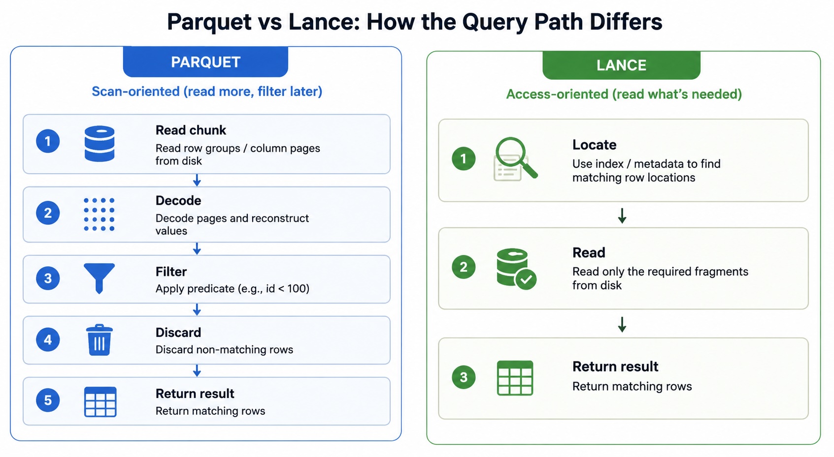
A compact way to visualize it is this:

Why Parquet Takes This Path

Parquet is not just a file of columns. Internally, a file is organized into row groups; each row group contains one column chunk per column, and column chunks are divided into pages, as described in the Parquet concepts and file format documentation. Parquet metadata also helps the reader skip some work before decoding begins, which is one of the format’s core strengths. See the metadata documentation. I covered the Parquet scan path in more detail in my earlier DZone article, Understanding Parquet Scans, so I’ll keep this recap focused on what changes in the read path as the workload becomes more selective.

[ repetition levels ]
[ definition levels ]
[ values ]

Those pages do not hold only values. They also hold structural information needed to reconstruct rows, especially when nested data is involved. This is also the lens used in the Lance paper. It argues that structural encoding, especially repetition, validity, and page layout, has a direct impact on random-access cost, read amplification, and decode overhead.

When a reader evaluates a predicate over Parquet data, it first uses metadata to decide which row groups may be relevant. It can skip some work at that level, which is one of Parquet’s strengths. But once a row group has been selected, the reader still needs to read column pages, decode them, reconstruct the row structure, and only then evaluate the filter.

That path is efficient when a query is scanning a large fraction of the dataset. It is less efficient when the result is tiny. The smallest useful unit of work is still a chunk.

This is why selective queries can feel disproportionately expensive in Parquet. The format is doing exactly what it was designed to do. It is just optimized around chunk-level processing rather than lookup-oriented access.

What Changes in Lance

Lance changes that path earlier.

Instead of treating most queries as scan-first, Lance uses dataset metadata and access structures to narrow the read before reconstruction begins. The official read and write guide is a good starting point for the dataset API used in the examples below. The reader can identify relevant fragments, read only the necessary data, and return results without paying the same chunk-level decode cost across the rest of the dataset.

For selective reads, the practical effect is that the reader can identify relevant fragments and avoid decoding larger portions of the dataset. For vector workloads, the index becomes even more important because the query is not looking for an exact predicate match. It is looking for nearby vectors.

That is the practical meaning behind the benchmark. The query returns 100 rows in both cases, but the amount of data processed before those rows are produced is different.

This distinction becomes clearer as the dataset grows because Parquet’s work still tracks chunk boundaries while Lance’s work is tied more closely to the size of the result.

Use Case 2: Vector Similarity

Filtered reads are still part of traditional analytics. Vector search is a different kind of workload.

A vector is just a list of numbers that represents something like text, an image, or a user. Instead of filtering by exact values, a system compares vectors and returns the nearest matches.

A traditional query looks for rows that satisfy a predicate. A vector query looks for rows that are similar.

In larger systems, vector search is usually implemented with an approximate nearest neighbor index, often called an ANN index. The index avoids comparing the query vector against every stored vector. Instead, it narrows the search to candidates that are likely to be close. This trades a small amount of exactness for much faster retrieval.

In many data lake architectures, this index lives outside the analytical dataset. Vectors may be stored in Parquet, then copied into a separate vector database or indexing service. That creates another pipeline to maintain and another consistency problem to manage.

This is why vector-native storage matters. The important change is not only that vectors can be stored. It is that retrieval becomes part of the dataset access path.

That difference sounds abstract until you tie it to something familiar. This shows up in semantic search, recommendations, LLM retrieval, and image similarity. In each case, the system is not looking for an exact value. It is looking for nearby representations.

The shape of the query changes from this:

WHERE id = 42 → exact match 

to this:

query → vector → nearest neighbors

That changes what the storage layer needs to support.

Here is the benchmark I used for the vector case:

import os
import shutil
import time

import numpy as np
import pandas as pd
import pyarrow as pa
import lance

# Try 1M, 5M, 10M to observe scaling behavior
N = 5_000_000

# Small result set -> stresses selective access vs scan
FILTER_EXPR = "id < 100"

# Run multiple times; use best to reduce noise
RUNS = 5


def clean_outputs():
    if os.path.exists("data.parquet"):
        os.remove("data.parquet")
    if os.path.exists("data.lance"):
        shutil.rmtree("data.lance")


def time_it(name, fn, runs=RUNS):
    times = []
    result = None

    for _ in range(runs):
        start = time.time()
        result = fn()
        times.append(time.time() - start)

    print(f"{name} times:", times)
    print(f"{name} best:", min(times))
    return result


def main():
    clean_outputs()

    print(f"Generating dataset with {N} rows...")

    df = pd.DataFrame({
        "id": np.arange(N),
        "value": np.random.rand(N)
    })

    # Parquet write (scan-optimized)
    start = time.time()
    df.to_parquet("data.parquet")
    print("Parquet write time:", time.time() - start)

    # Lance write (Arrow-based)
    start = time.time()
    table = pa.Table.from_pandas(df)
    lance.write_dataset(table, "data.lance", mode="overwrite")
    print("Lance write time:", time.time() - start)

    dataset = lance.dataset("data.lance")

    # Selective filter: returns ~100 rows
    result_parquet = time_it(
        "Parquet filter",
        lambda: pd.read_parquet("data.parquet").query(FILTER_EXPR)
    )

    result_lance = time_it(
        "Lance filter",
        lambda: dataset.to_table(filter=FILTER_EXPR).to_pandas()
    )

    print("Parquet rows:", len(result_parquet))
    print("Lance rows:", len(result_lance))


if __name__ == "__main__":
    main() 

Here is a sample run from my laptop:

(parquet-lance-demo) hitarth@hitarth parquet_lance % python vector.py 
Generating 100000 vectors of dimension 128...
Lance write time: 0.07955217361450195
Vector search time: 0.13872408866882324
      id                                             vector  _distance
0  50506  [0.053919002, 0.36111426, 0.2145877, 0.9197419...  12.631166
1  41428  [0.17633885, 0.71251565, 0.072742924, 0.759959...  12.962575
2   3216  [0.06450701, 0.24716537, 0.41617322, 0.624773,...  13.008584
3  50216  [0.13460344, 0.9618073, 0.8334099, 0.56230646,...  13.097234
4  75019  [0.35094073, 0.11819457, 0.44928855, 0.0426102...  13.124901

This wrote 100,000 vectors of dimension 128 and returned the top 5 nearest vectors in about 139 ms. The exact number is less important than the query path itself: the search runs directly against the dataset and returns nearest neighbors with distances.

Parquet can store the same vector column, but it does not provide a native nearest-neighbor query path. In practice, the workflow usually looks like this:

Parquet → extract vectors → build index → query

With Lance, the storage layer participates directly in the query:

dataset → query directly

That is not just a performance difference. It is a capability difference.

Lance’s official documentation also exposes SDK-level APIs for working with datasets and vector-oriented workflows through the SDK docs.  Lance expects vector columns as fixed-size arrays rather than generic variable-length Python lists. That lets the system reason about dimensionality during query execution. In other words, the structure of the stored data is part of making the query possible.

Tradeoffs and Operational Considerations

This comparison should not be read as "Lance replaces Parquet." The two formats are useful in different parts of a data platform.

Parquet remains the safer default for broad analytical workloads. It has mature support across query engines, data lakes, catalogs, ingestion systems, and governance tooling. If the workload is mostly batch analytics, reporting, or large aggregations, Parquet’s scan-oriented design is still a very good fit.

Lance becomes interesting when the workload starts to depend on repeated selective access, lower-latency retrieval, or vector-native queries. In those cases, avoiding unnecessary decoding or avoiding a separate vector indexing pipeline can matter more than raw scan throughput.

A simplified comparison looks like this:

The operational question is not which format is generally better. The better question is where the workload spends its time. If most queries scan large portions of data, Parquet is still the right default. If the workload repeatedly asks for a small number of rows or nearest neighbors, a lookup-oriented or vector-native format becomes more attractive.

What the Two Examples Show Together

The filtered read example and the vector example highlight two different consequences of the same design choice. 

In the filtered read case, the difference appears as execution cost. Both systems can answer the query, but the amount of data processed before returning the result is different.

In the vector case, the difference appears as capability. One format stores the data, while the other format also provides a native query path over it.

Both cases come back to the same question: how much data must the system process before it can produce the answer?

For scan-heavy analytics, Parquet remains a strong fit. That is the read path it was built for. But when workloads shift toward selective access, repeated reads, or similarity search, the main question changes. The difference is no longer just how fast data can be scanned. It is how much data the reader must process before returning the result.

That is the broader storage trend. File formats are becoming more involved in the read path itself. They increasingly encode assumptions about access patterns, indexing, and retrieval. As analytical, ML, and search workloads move closer together, storage layout becomes part of query design.