Practitioner’s Guide to Deep Learning
An overview of best practices, recommendations, and fundamentals for managing a deep learning project to ensure a robust AI product.
Join the DZone community and get the full member experience.
Join For FreeOur world is undergoing an AI revolution powered by very deep neural networks. With the advent of Apple Intelligence and Gemini, AI has reached the hands of every human being with a mobile phone. Apart from consumer AI, we also have deep learning models being used in several industries like automobile, finance, medical science, manufacturing, etc. This has motivated many engineers to learn deep learning techniques and apply them to solve complex problems in their projects. In order to help these engineers, it becomes imperative to lay down certain guiding principles to prevent common pitfalls when building these black box models.
Any deep learning project involves five basic elements: data, model architecture, loss functions, optimizer, and evaluation process. It is critical to design and configure each of these appropriately to ensure proper convergence of models. This article shall cover some of the recommended practices and common problems and their solutions associated with each of these elements.
Data
All deep-learning models are data-hungry and require several thousands of examples at a minimum to reach their full potential. To begin with, it is important to identify the different sources of data and devise a proper mechanism for selecting and labeling data if required. It helps to build some heuristics for data selection and gives careful consideration to balance the data to prevent unintentional biases. For instance, if we are building an application for face detection, it is important to ensure that there is no racial or gender bias in the data, as well as the data is captured under different environmental conditions to ensure model robustness. Data augmentations for brightness, contrast, lighting conditions, random crop, and random flip also help to ensure proper data coverage.
The next step is to carefully split the data into train, validation, and test sets while ensuring that there is no data leakage. The data splits should have similar data distributions but identical, or very closely related samples should not be present in both train and test sets. This is important, as if train samples are present in the test set, then we may see high test performance metrics but still several unexplained critical issues in production. Also, data leakage makes it almost impossible to know if the alternate ideas for model improvement are bringing about any real improvement or not. Thus, a diverse, leak-proof, balanced test dataset representative of the production environment is your best safeguard to deliver a robust deep learning-based model and product.
Model Architecture
In order to get started with model design, it makes sense to first identify the latency and performance requirements of the task at hand. Then, one can look at open-source benchmarks like this one to identify some suitable papers to work with. Whether we use CNNs or transformers, it helps to have some pre-trained weights to start with, to reduce training time. If no pre-trained weights are available, then suitable model initialization for each model layer is important to ensure that the model converges in a reasonable time. Also, if the dataset available is quite small (a few hundred samples or less), then it doesn’t make sense to train the whole model, rather just the last few task-specific layers should be fine-tuned.
Now, whether to use CNN, transformers, or a combination of them is very specific to the problem. For natural language processing, transformers have been established as the best choice. For vision, if the latency budget is very tight, CNNs are still the better choice; otherwise, both CNNs and transformers should be experimented with to get the desired results.
Loss Functions
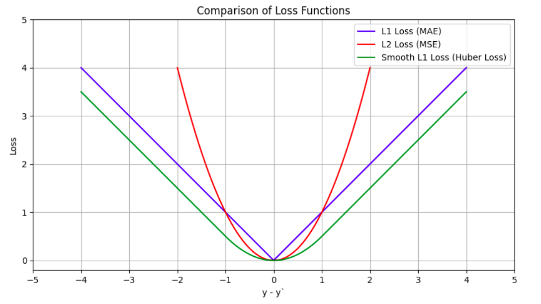
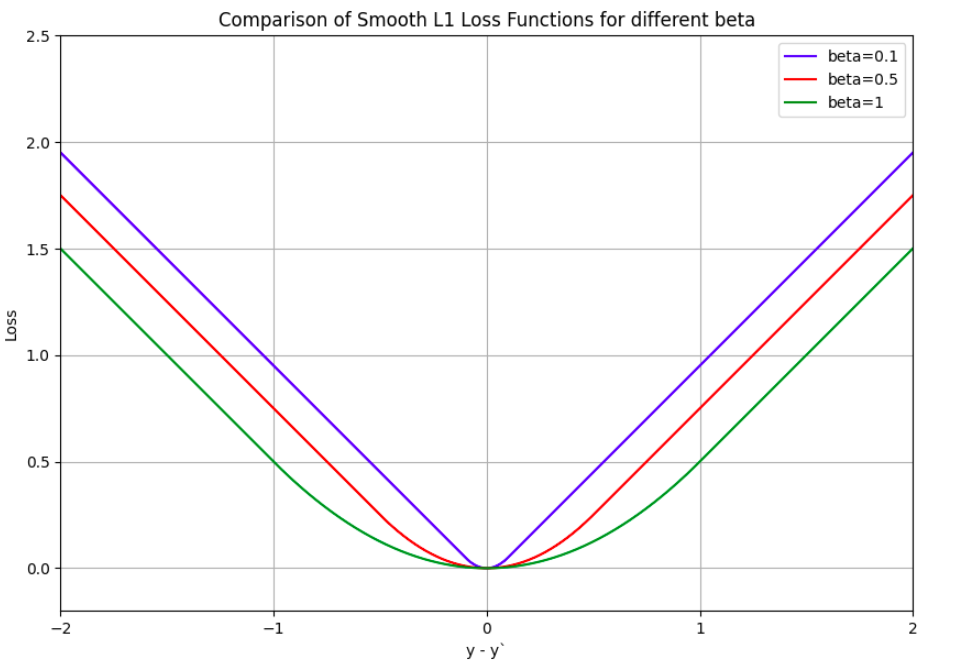
The most popular loss function for classification tasks is the Cross Entropy Loss and for regression tasks are the L1 or L2 (MSE) losses. However, there are certain variations of them available for numerical stability during model training. For instance in Pytorch, BCEWithLogitsLoss combines the sigmoid layer and BCELoss into a single class and uses the log-sum-exp trick which makes it more numerically stable than a sigmoid layer followed by BCELoss. Another example is of SmoothL1Loss which can be seen as a combination of L1 and L2 loss and makes the L1 Loss smooth near zero. However, care must be taken when using smooth L1 Loss to set the beta appropriately as its default value of 1.0 may not be suitable for regressing values in sine and cosine domains. The figures below show the loss values for L1, L2 (MSE), and Smooth L1 losses and also the change in smooth L1 Loss value for different beta values.


Optimizer
Stochastic Gradient Descent with momentum has traditionally been a very popular optimizer among researchers for most problems. However, in practice, Adam is generally easier to use but suffers from generalization problems. Transformer papers have popularized the AdamW optimizer which decouples the weight-decay factor’s choice from the learning rate and significantly improves the generalization ability of Adam optimizer. This has made AdamW the optimal choice for optimizers these days.
Also, it isn’t necessary to use the same learning rate for the whole network. Generally, if starting from a pre-trained checkpoint, it is better to freeze or keep a low learning rate for the initial layers and a higher learning rate for the deeper task-specific layers.
Evaluation and Generalization
Developing a proper framework for evaluating the model is the key to preventing issues in production. This should involve both quantitative and qualitative metrics for not only the full benchmark dataset but also for specific scenarios. This should be done to ensure that performance is acceptable in every scenario and there is no regression.
Performance metrics should be carefully chosen to ensure that they appropriately represent the task to be achieved. For example, precision/recall or F1 score may be better than accuracy in many unbalanced problems. At times, we may have several metrics to compare alternate models, then it generally helps to come up with a single weighted metric that can simplify the comparison process. For instance, the nuScenes dataset introduced NDS (nuScenes Detection Score) which is a weighted sum of mAP (mean average precision), mATE (mean average translation error), mASE (mean average scale error), mAOE(mean average orientation error), mAVE(mean average velocity error) and mAAE(mean average attribute error) to simplify comparison of various 3D object detection models.
Further, one should also visualize the model outputs whenever possible. This could involve drawing bounding boxes on input images for 2D object detection models or plotting cuboids on LIDAR point clouds for 3D object detection models. This manual verification ensures that model outputs are reasonable and there is no apparent pattern in model errors.
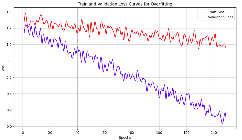
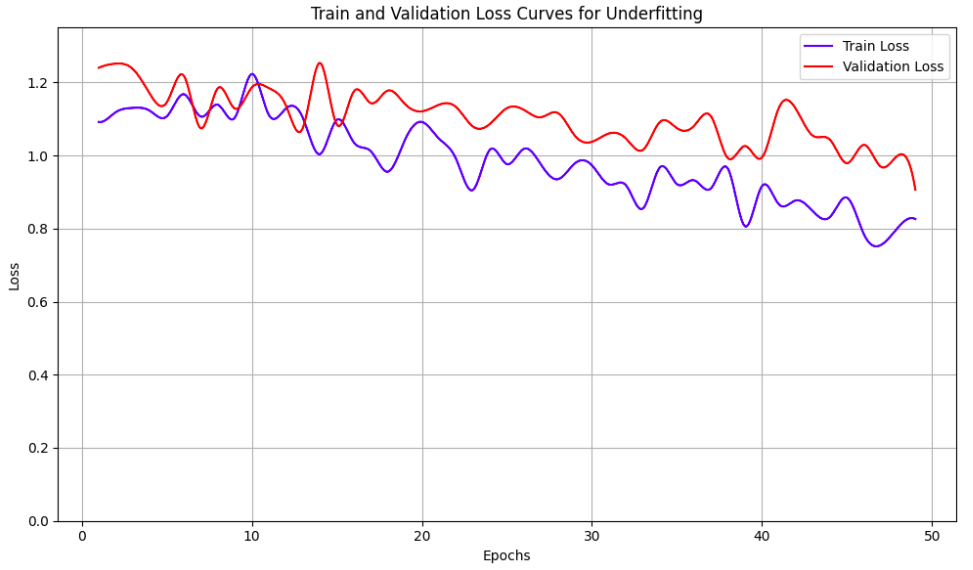
Additionally, it helps to pay close attention to training and validation loss curves to check for overfitting or underfitting. Overfitting is a problem wherein validation loss diverges from training loss and starts increasing, representing that the model is not generalizing well. This problem can generally be fixed by adding proper regularization like weight-decay, drop-out layers, adding more data augmentation, or by using early stopping. Underfitting, on the other hand, represents the case where the model doesn’t have enough capacity to even fit the training data. This can be identified by the training loss not going down enough and/or remaining more or less flat over the epochs. This problem can be addressed by adding more layers to the model, reducing data augmentations, or selecting a different model architecture. The figures below show examples of overfitting and underfitting through the loss curves.


The Deep Learning Journey
Unlike traditional software engineering, deep learning is more experimental and requires careful tuning of hyper-parameters. However, if the fundamentals mentioned above are taken care of, this process can be more manageable. Since the models are black boxes, we have to leverage the loss curves, output visualizations, and performance metrics to understand model behavior and correspondingly take corrective measures. Hopefully, this guide can make your deep learning journey a little less taxing.
Opinions expressed by DZone contributors are their own.

Comments