

Real-Time Vehicle Tracking With Neo4j, Databricks Lakebase, and OpenStreetMap
Build a real-time fleet operations dashboard using Neo4j Aura for the road network graph, Lakebase for live vehicle positions, and Lakehouse for historical analytics.
 CORE
·
CORE
·
Join the DZone community and get the full member experience.
Join For FreeMost vehicle tracking systems ask one database to do everything. For example, store the road network, query it with recursive CTEs, write live positions to the same database, run analytics on the same tables, and so on. It works until the graph queries slow down, high-frequency writes start competing with reads, and analytics queries time out.
This article shows a different approach: three databases, each doing what it's genuinely good at. Neo4j Aura for the road network graph, Databricks Lakebase for live vehicle positions, and Databricks Lakehouse for historical analytics. Ten simulated vehicles move around a real city following real road connections loaded from OpenStreetMap. Two Streamlit dashboards show live positions and analytics. The whole system is driven by a single YAML configuration file, so switching from London to San Francisco or Singapore means changing a single file and rerunning five notebooks.
The full source code is available on GitHub.
The Three-System Architecture
The architecture has three distinct layers:
- Neo4j Aura holds the road network — intersections, road segments, zone topology, and shortest paths. It answers graph questions that a relational database may handle awkwardly.
- Databricks Lakebase holds the live operational data — vehicle positions written every two seconds by a simulator, vehicle statuses, and trip records. It's a fully managed Postgres database inside Databricks, handling OLTP workloads with standard
psycopg2connectivity. - Databricks Lakehouse holds the analytical history — position data synced from Lakebase into a Delta table, aggregated by zone and road segment.
None of these systems knows about the others. The intelligence sits in the application layer — the simulator, the Streamlit dashboards and the analytics notebook — which orchestrates queries across all three and combines the results.
The Road Network in Aura
We'll use OSMnx to download the drivable road network for the London Borough of Merton from OpenStreetMap and load it into Aura. The graph model is straightforward:
(:Intersection {node_id, lat, lon, street_count, location})
    -[:ROAD {osmid, name, highway, maxspeed, oneway, length_m}]->
(:Intersection)
Merton's road network produces thousands of intersection nodes and thousands of directed road relationships. A POINT INDEX on the location property enables fast nearest-neighbor lookups -- finding the intersection closest to any GPS coordinate runs in milliseconds.
The reason for Aura is simple: the road network is a graph and graph queries are where Aura excels. Finding the shortest path between two zones is a single Cypher function call:
MATCH path = shortestPath((start)-[:ROAD*..300]->(end))
RETURN length(path) AS hops
The equivalent in SQL requires a recursive CTE that grows in complexity with every additional hop. For zone reachability queries — "which zones can a vehicle reach within two hops?" — the difference is even more pronounced.
We also define five logical zones as bounding boxes within the borough and store them as Zone nodes with ADJACENT_TO relationships. This gives us a zone adjacency graph that the simulator uses for routing decisions.
The Simulator
The simulator loads the entire road graph from Aura into memory at startup — one query, one dictionary, no further Aura calls during the simulation loop. It then places ten vehicles at their home intersections and moves each one along Breadth-First Search (BFS)-computed routes.
Vehicles don't route randomly. They have a home zone and a 70% chance of staying in or near it. The remaining 30% of the time, they cross into any zone in the borough, producing occasional longer cross-city runs. Every two seconds, each vehicle writes its current coordinates to Lakebase:
cursor.execute("""
    INSERT INTO vehicle_positions
        (vehicle_id, lat, lon, speed_kmh, current_zone)
    VALUES (%s, %s, %s, %s, %s)
""", (vehicle_id, lat, lon, speed_kmh, current_zone))
The simulator runs as a background subprocess launched from a Jupyter notebook, continuing independently while the Streamlit dashboards are open.
The Live Vehicle Tracker
The vehicle tracker (app.py) refreshes every three seconds and shows three pydeck layers on a CARTO basemap:
- Vehicle icons – one car icon per vehicle at its current GPS position
- Trail lines – each vehicle's last 20 positions, colored by home zone
- Shortest path – a black line showing the road-network shortest path between any two selected zones, computed on demand from Aura
Figure 1 shows vehicles moving on the Merton map with trail lines and a shortest path highlighted between two zones.
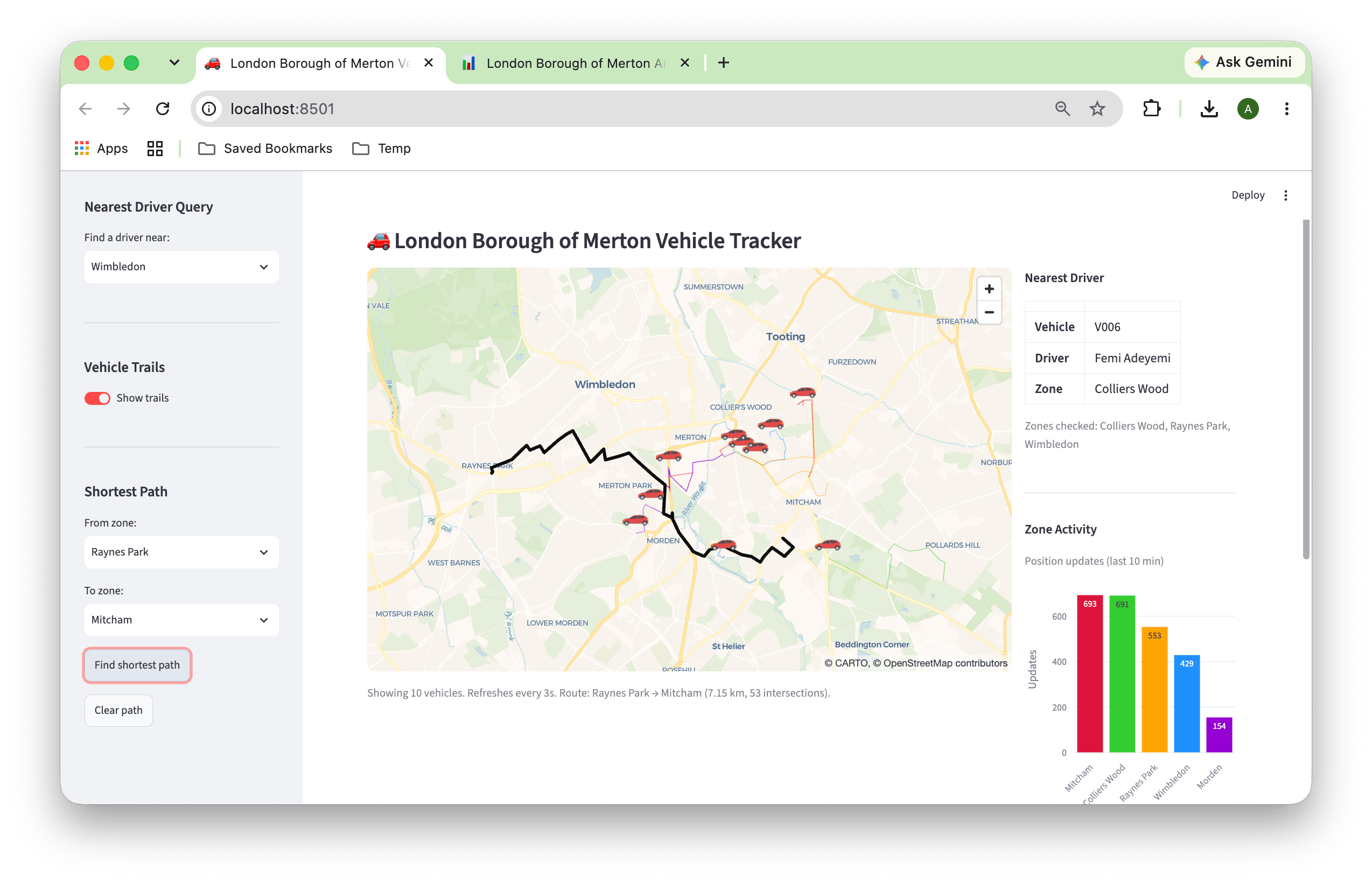
Figure 1. Streamlit Vehicle Tracker.
The sidebar shows a bar chart of zone activity over the last 10 minutes and a nearest-driver lookup -- given a zone, which vehicle is currently closest to it? The haversine distance calculation runs against the latest position of every vehicle, using zone center coordinates that map to real road intersections.
The Analytics Dashboard
The analytics dashboard (analytics_app.py) connects to all three systems simultaneously. Every 30 seconds, it syncs new position records from Lakebase into a Lakehouse Delta table and runs two analytical queries.
Figure 2 shows an analytics dashboard with zone activity over time across all five zones.
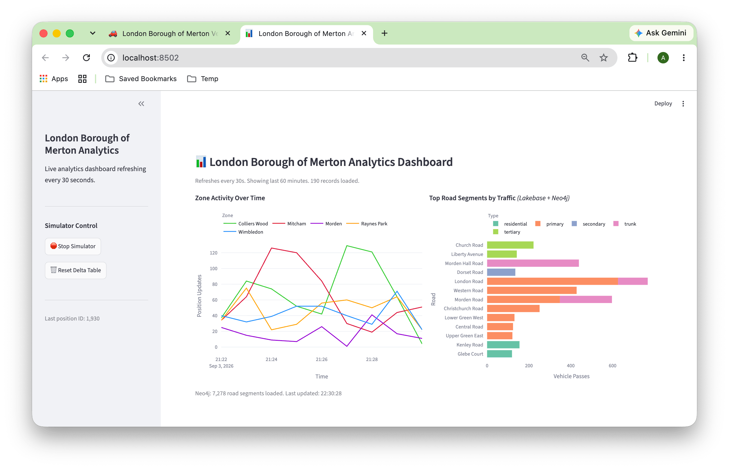
Figure 2. Analytics Dashboard.
The chart on the left-hand side shows position update counts per zone per minute over the last hour — a live view of which parts of the city are busiest:
SELECT current_zone AS zone,
       DATE_TRUNC('minute', recorded_at) AS minute,
       COUNT(*) AS updates
FROM vehicle_positions_delta
WHERE current_zone IS NOT NULL
GROUP BY current_zone, DATE_TRUNC('minute', recorded_at)
ORDER BY minute, zone
The chart on the right-hand side is the architectural highlight: a cross-system join that answers "which named roads carry the most vehicle traffic?" Lakebase has the position records (latitude, longitude, per vehicle per tick). Aura has the road names (what named road each intersection belongs to). Neither system alone can answer the question.
The join runs in Python using pandas. Road names and coordinates are loaded from Aura once at startup and cached. Position coordinates come from Lakebase via the Lakehouse Delta table on each refresh. Coordinates are rounded to three decimal places (~100m precision) and joined:
joined = pos_df.merge(
    road_df[["road_name", "highway", "lat_r", "lon_r"]],
    on=["lat_r", "lon_r"],
    how="inner"
)
Primary roads dominate because BFS routing naturally follows main roads when finding shortest paths.
The YAML Configuration System
Every city-specific value lives in a single config.yaml file which contains zone definitions, vehicle assignments, map coordinates, and the OpenStreetMap place name.
city:
  name: "London Borough of Merton"
  osmnx_place: "London Borough of Merton, UK"
  network_type: "drive"
  map_lat: 51.410
  map_lon: -0.188
  map_zoom: 12
Switching cities means copying a different config file and re-running five notebooks. Three example config files are included: Merton (London), San Francisco, and Singapore. For cities where OSMnx's place name geocoding doesn't produce a usable polygon boundary, a pyrosm-based approach clips a Geofabrik regional file to a bounding box instead. The pre-clipped files for San Francisco and Singapore are included in the GitHub repo, so you can run those configs without any additional data preparation.
A companion config_validator.py validates the file on load and raises clear errors if anything is missing or malformed.
Why Three Systems?
The answer is that each system does something the others can't do efficiently.
Neo4j Aura handles graph traversals — shortest paths, multi-hop reachability, nearest-node spatial lookups. These are awkward in SQL and natural in Cypher.
Databricks Lakebase handles high-frequency OLTP writes — hundreds of inserts per minute, sustained, with foreign key constraints and BIGSERIAL auto-increment.
Databricks Lakehouse handles analytical aggregations over historical data — counting position records by zone and minute, joining across large datasets. Columnar storage and parallel execution make this fast.
The three-system architecture isn't complexity for its own sake. Each system earns its place by doing something the others would handle poorly.
The Free Online Book
The full system — all notebooks, both Streamlit apps, the YAML config system and seven chapters of detailed explanation — is available as a free online book.
The book covers the road network loading and data cleaning, zone and adjacency graph setup, Lakebase table design, the BFS simulator, both Streamlit dashboards, the analytics notebook, and all the gotchas and lessons learned. The code is on GitHub under Apache 2.0. The pre-clipped OSM data files are available under the Open Database License (ODbL).
Summary
We've built a real-time fleet operations dashboard using three database systems, each doing what it does best: Neo4j Aura for road network graph queries and shortest path computation, Databricks Lakebase for high-frequency vehicle position writes, and Databricks Lakehouse for historical analytics over Delta tables. The interesting engineering is in the joins that cross system boundaries — finding the nearest driver uses Aura's spatial index, routing vehicles uses BFS over an in-memory graph loaded from Aura, and identifying the busiest named roads joins position data with road names via pandas. A YAML configuration file drives the entire system, making it straightforward to point the same codebase at a different city. The architecture demonstrates that a multi-database approach isn't inherently complex — it becomes simpler when each system has a clear, non-overlapping role.
The full source code is available on GitHub.
Opinions expressed by DZone contributors are their own.
Comments