Unboxing the Black Box

Today, several significant and safety-critical decisions are being made by deep neural networks. These include driving decisions in autonomous vehicles, diagnosing diseases, and operating robots in manufacturing and construction. In all such cases, scientists and engineers claim that these models help make better decisions than humans and hence, help save lives. However, how these networks reach their decisions is often a mystery, for not just their users, but also for their developers. 

These changing times, thus, necessitate that as engineers we spend more time unboxing these black boxes so that we can identify the biases and weaknesses of the models that we build. This may also allow us to identify which part of the input is most critical for the model and hence, ensure its correctness. Finally, explaining how models make their decisions will not only build trust between AI products and their consumers but also help meet the diverse and evolving regulatory requirements.

The whole field of explainable AI is dedicated to figuring out the decision-making process of models. In this article, I wish to discuss some of the prominent explanation methods for understanding how computer vision models arrive at a decision. These techniques can also be used to debug models or to analyze the importance of different components of the model. 

The most common way to understand model predictions is to visualize heat maps of layers close to the prediction layer. These heat maps when projected on the image allow us to understand which parts of the image contribute more to the model’s decision. Heat maps can be generated either using gradient-based methods like CAM, or Grad-CAM or perturbation-based methods like I-GOS or I-GOS++. A bridge between these two approaches, Score-CAM, uses the increase in model confidence scores to provide a more intuitive way of generating heat maps. In contrast to these techniques, another class of papers argues that these models are too complex for us to expect just a single explanation for their decision. Most significant among these papers is the Structured Attention Graphs method which generates a tree to provide multiple possible explanations for a model to reach its decision. 

Class Activation Map (CAM) Based Approaches

1. CAM

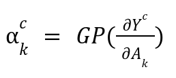
Class Activation Map (CAM) is a technique for explaining the decision-making of specific types of image classification models. Such models have their final layers consisting of a convolutional layer followed by global average pooling, and a fully connected layer to predict the class confidence scores. This technique identifies the important regions of the image by taking a weighted linear combination of the activation maps of the final convolutional layer. The weight of each channel comes from its associated weight in the following fully connected layer. It's quite a simple technique but since it works for a very specific architectural design, its application is limited. Mathematically, the CAM approach for a specific class c can be written as:

where
is the weight for activation map (A) of the kth channel of the convolutional layer.

ReLU is used as only positive contributions of the activation maps are of interest for generating the heat map.

2. Grad-CAM

The next step in CAM evolution came through Grad-CAM, which generalized the CAM approach to a wider variety of CNN architectures. Instead of using the weights of the last fully connected layer, it determines the gradient flowing into the last convolutional layer and uses that as its weight. So for the convolutional layer of interest A, and a specific class c, they compute the gradient of the score for class c with respect to the feature map activations of a convolutional layer. Then, this gradient is the global average pooled to obtain the weights for the activation map.

The final obtained heat map is of the same shape as the feature map output of that layer, so it can be quite coarse. Grad-CAM maps become progressively worse as we move to more initial layers due to reducing receptive fields of the initial layers. Also, gradient-based methods suffer from vanishing gradients due to the saturation of sigmoid layers or zero-gradient regions of the ReLU function. 

3. Score-CAM

Score-CAM addresses some of these shortcomings of Grad-CAM by using Channel-wise Increase of Confidence (CIC) as the weight for the activation maps. Since it does not use gradients, all gradient-related shortcomings are eliminated. Channel-wise Increase of Confidence is computed by following the steps below:

1. Upsampling the channel activation maps to input size and then, normalizing them
2. Then, computing the pixel-wise product of the normalized maps and the input image
3. Followed by taking the difference of the model output for the above input tensors and some base images which gives an increase in confidence
4. Finally, applying softmax to normalize the activation maps weights to [0, 1]

The Score-CAM approach can be applied to any layer of the model and provides one of the most reasonable heat maps among the CAM approaches.

In order to illustrate the heat maps generated by Grad-CAM and Score-CAM approaches, I selected three images: bison, camel, and school bus images. For the model, I used the Convnext-Tiny implementation in TorchVision. I extended the PyTorch Grad-CAM repo to generate heat maps for the layer convnext_tiny.features[7][2].block[5]. From the visualization below, one can observe that Grad-CAM and Score-CAM highlight similar regions for the bison image. However, Score-CAM’s heat map seems to be more intuitive for the camel and school bus examples.

Perturbation-Based Approaches

Perturbation-based approaches work by masking part of the input image and then observing how this affects the model's performance. These techniques directly solve an optimization problem to determine the mask that can best explain the model’s behavior. I-GOS and I-GOS++ are the most popular techniques under this category. 

1. Integrated Gradients Optimized Saliency (I-GOS)

The I-GOS paper generates a heat map by finding the smallest and smoothest mask that optimizes for the deletion metric. This involves identifying a mask such that if the masked portions of the image are removed, the model's prediction confidence will be significantly reduced. Thus, the masked region is critical for the model’s decision-making.

The mask in I-GOS is obtained by finding a solution to an optimization problem. One way to solve this optimization problem is by applying conventional gradients in the gradient descent algorithm. However, such a method can be very time-consuming and is prone to getting stuck in local optima. Thus, instead of using conventional gradients, the authors recommend using integrated gradients to provide a better descent direction. Integrated gradients are calculated by going from a baseline image (giving very low confidence in model outputs) to the original image and accumulating gradients on images along this line.

2. I-GOS++

I-GOS++ extends I-GOS by also optimizing for the insertion metric. This metric implies that only keeping the highlighted portions of the heat map should be sufficient for the model to retain confidence in its decision. The main argument for incorporating insertion masks is to prevent adversarial masks which don’t explain the model behavior but are very good at deletion metrics. In fact, I-GOS++ tries to optimize for three masks: a deletion mask, an insertion mask, and a combined mask. The combined mask is the dot product of the insertion and deletion masks and is the output of the I-GOS++ technique. This technique also adds regularization to make masks smooth on image areas with similar colors, thus enabling the generation of better high-resolution heat maps. 

Next, we compare the heat maps of I-GOS and I-GOS++ with Grad-CAM and Score-CAM approaches. For this, I made use of the I-GOS++ repo to generate heat maps for the Convnext-Tiny model for the bison, camel, and school bus examples used above. One can notice in the visualization below that the perturbation techniques provide less diffused heat maps compared to the CAM approaches. In particular, I-GOS++ provides very precise heat maps. 

Structured Attention Graphs for Image Classification

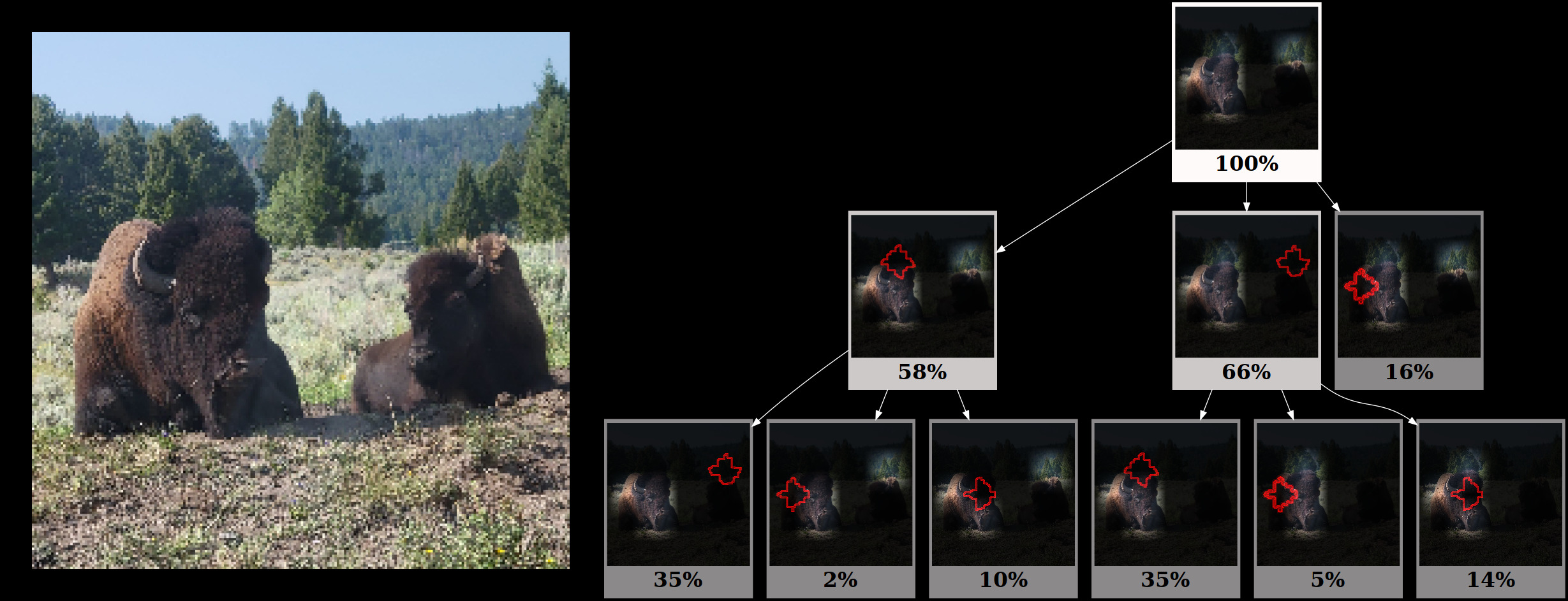
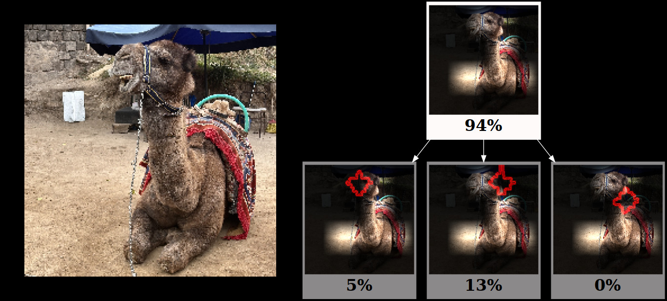
The Structured Attention Graphs (SAG) paper presents a counter view that a single explanation (heat map) is not sufficient to explain a model's decision-making. Rather multiple possible explanations exist which can also explain the model’s decision equally well. Thus, the authors suggest using beam-search to find all such possible explanations and then using SAGs to concisely present this information for easier analysis. SAGs are basically “directed acyclic graphs” where each node is an image patch and each edge represents a subset relationship. Each subset is obtained by removing one patch from the root node’s image. Each root node represents one of the possible explanations for the model’s decision.

To build the SAG, we need to solve a subset selection problem to identify a diverse set of candidates that can serve as the root nodes. The child nodes are obtained by recursively removing one patch from the parent node. Then, the scores for each node are obtained by passing the image represented by that node through the model. Nodes below a certain threshold (40%) are not expanded further. This leads to a meaningful and concise representation of the model's decision-making process. However, the SAG approach is limited to only coarser representations as combinatorial search is very computationally expensive.

Some illustrations for Structured Attention Graphs are provided below using the SAG GitHub repo. For the bison and camel examples for the Convnext-Tiny model, we only get one explanation; but for the school bus example, we get 3 independent explanations. 

Applications of Explanation Methods

Model Debugging

The I-GOS++ paper presents an interesting case study substantiating the need for model explainability. The model in this study was trained to detect COVID-19 cases using chest x-ray images. However, using the I-GOS++ technique, the authors discovered a bug in the decision-making process of the model. The model was paying attention not only to the area in the lungs but also to the text written on X-ray images. Obviously, the text should not have been considered by the model, indicating a possible case of overfitting. To alleviate this issue, the authors pre-processed the images to remove the text and this improved the performance of the original diagnosis task. Thus, a model explainability technique, IGOS++ helped debug a critical model.

Understanding Decision-Making Mechanisms of CNNs and Transformers

Jiang et. al. in their CVPR 2024 paper, deployed SAG, I-GOS++, and Score-CAM techniques to understand the decision-making mechanism of the most popular types of networks: Convolutional Neural Networks (CNNs) and Transformers. This paper applied explanation methods on a dataset basis instead of a single image and gathered statistics to explain the decision-making of these models. Using this approach, they found that Transformers have the ability to use multiple parts of an image to reach their decisions in contrast to CNNs which use several disjoint smaller sets of patches of images to reach their decision.

Key Takeaways

• Several heat map techniques like Grad-CAM, Score-CAM, IGOS, and IGOS++ can be used to generate visualizations to understand which parts of the image a model focuses on when making its decisions.
• Structured Attention Graphs provide an alternate visualization to provide multiple possible explanations for the model’s confidence in its predicted class.
• Explanation techniques can be used to debug the models and can also help better understand model architectures.