A Deep Dive Into Couchbase N1QL Query Optimization
This comprehensive guide to N1QL queries covers the ins and outs of the query engine, teaching users about how to efficiently scan and join data.
Join the DZone community and get the full member experience.
Join For FreeSQL is the declarative language for manipulating data in a relational database system. N1QL is the declarative language for JSON data and metadata. Similar to SQL, N1QL has DML statements to manipulate JSON data: SELECT, INSERT, UPDATE, DELETE, MERGE, EXPLAIN. It also introduces a new statement, INFER, which samples the data to describe the schema and show data samples.
Execution of a N1QL query by the engine involves multiple steps. Understanding these will help you to write queries, design for performance, tune query engine efficiently. The N1QL query engine includes parser, semantic analyzer, optimizer and executor. This article will describe how the N1QL query optimizer creates the query plan.
Life of a Query: Overview
Applications and their drivers submit the N1QL query to one of the available query nodes in the Couchbase cluster. The query node analyzes the query, uses metadata on underlying objects to to create the execution plan, executes it. During execution, the query node orchestrates with index and data nodes to perform the select-join-nest-unnest-project operations.
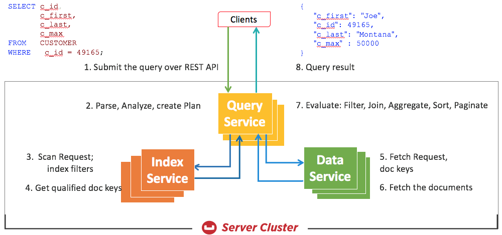
Inside a Query Node
Within each query service, the query flows through the different stages shown below. The N1QL parser checks for syntactic correctness, and the semantic analyzer ensures that the query is meaningful. The N1QL optimizer takes the parsed tree as input, selects suitable indexes, selects access paths for each object and then creates the query plan. It's from this plan that an execution tree with all the necessary operators is created. The execution tree is then executed to manipulate the data, project query results.
N1QL Query Optimizer
Every flight has a flight plan before it takes off. Each flight has many options for its route. But, depending on guidelines, weather, best practices, and regulations, they decide on a specific flight plan.
Every N1QL query has a query plan. Just like a flight plan, each query can be executed in many ways — different indexes to choose, different predicates to push down, different orders of joins, etc. Eventually, the N1QL query engine will choose an access path in each case and come up with the plan. This plan is converted to query execution tree. This stage of query execution is called optimization.
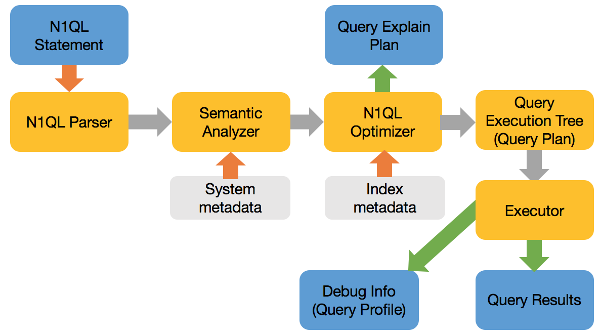
The figure below shows all the possible phases a query goes through during execution to return the results. Not all queries need to go through every phase. Some go through many of these phases multiple times. Optimizer decides phases each queries executes. For example, the Sort phase will be skipped when there is no ORDER BY clause in the query; the scan-fetch-join phase executes multiple times to perform multiple joins.

Some operations, like query parsing and planning, are done serially — denoted by a single block in the figure. Operations like fetch, join, or sort are done in parallel — denoted by multiple blocks in the figure.
N1QL optimizer analyzes the query and comes up with available access path options for each keyspace in the query. The planner needs to first select the access path for each keyspace, determine the join order and then determine the type of the join. This is done for each query block. Once the plans are done for all the query blocks, the execution is created.
The query below has two keyspaces, airline and airport:
SELECT airline, airport
FROM `travel-sample` airline
         INNER JOIN `travel-sample airport
                ON KEYS airline.airport_id
WHERE airline.type = ‘airline’
AND airport.type = ‘airports’
Access Path Selection
Keyspace (Bucket) access path options:
Keyscan access. When specific document IDs (keys) are available, the Keyscan access method retrieves those documents. Any filters on that keyspace are applied on those documents. The Keyscan can be used when a keyspace is queried by specifying the document keys (USE KEYS modifier) or during join processing. The Keyscan is commonly used to retrieve qualifying documents on for the inner keyspace during join processing.
PrimaryScan access: This is equivalent of a full table scan in relational database systems. This method is chosen when documents IDs are not given and no qualifying secondary indexes are available for this keyspace. N1QL will retrieve all of document IDs from the primary index, fetch the document and then do the predicate-join-project processing. This access method is quite expensive and the average time to return results increases linearly with number of documents in the bucket. Many customers use primary scan while developing the application, but drop the primary index altogether during production deployment. Couchbase or N1QL does not require the primary index as long as the query has a viable index to access the data.
IndexScan access: A qualifying secondary index scan is used to first filter the keyspace and to determine the qualifying documents IDs. It then retrieves the qualified documents from the data store, if necessary. If the selected index has all the data to answer the query, N1QL avoids fetching the document altogether — this method is called the covering index scan. This is highly performant. Your secondary indexes should help queries choose covering index scans as much as possible.
In Couchbase, the secondary index can be a standard global secondary index using ForestDB or Memory Optimized Index(MOI).
Index Selection
Here is the approach to select the secondary indexes for the query. The N1QL planner determines qualified indexes on the keyspace based on query predicates. The following is the algorithm to select the indexes for a given query.
Online indexes: Only online indexes are selected. That means when the indexes are being built (pending) or only defined, but not built, they aren't chosen.
Preferred indexes: When a statement has the USE INDEX clause, it provides the list of indices to consider. In this case, only those indices are evaluated.
Satisfying index condition: Partial indexes (when the index creation includes the WHERE clause) with a condition that is a super set of the query predicate are selected
Satisfying index keys: Indexes whose leading keys satisfy query predicate are selected. This is the common way to select indexes with B-TREE indexes.
Longest satisfying index keys: Redundancy is eliminated by keeping longest satisfying index keys in the index key order. For example, Index with satisfying keys (a, b, c) is retained over index with satisfying (a, b).
Once the index selection is done the following scan methods are considered in the order.
IndexCountScan
Queries with a single projection of COUNT aggregate, NO JOINs, or GROUP BY are considered. The chosen index needs to be covered with a single exact range for the given predicate, and the argument to COUNT needs to be constant or leading key.
Covering secondary scan
Each satisfied index with the most number of index keys is examined for query coverage, and the shortest covering index will be used. For an index to cover the query, we should be able to run the complete query just using the data in the index. In other words, the index needs to have both keys in the predicate as well as the keys referenced in other clauses, e.g., projection, subquery, order by, etc.
Regular secondary scan
Indexes with the most number of matching index keys are used. When more than one index is qualified, IntersectScan is used. To avoid IntersectScan, provide a hint with USE INDEX.
UNNEST Scan
Only array indexes with an index key matching the predicates are used for UNNEST scan.
Regular primary scan
If a primary scan is selected, and no primary index available, the query errors out.
JOIN Methods
N1QL supports nested loop access method for all the join supports: INNER JOIN and LEFT OUTER JOIN and the index join method.
Here is the simplest explanation of the join method.
For this join, ORDERS become the outer keyspace and CUSTOMER becomes the inner keyspace. The ORDERS keyspace is scanned first (using one of the keyspace scan options). For each qualifying document on ORDERS, we do a KEYSCAN on CUSTOMER based on the key O_C_D in the ORDERS document.
SELECT *
FROM ORDERS o INNER JOIN CUSTOMER c ON KEYS o.O_C_ID;
Index Join
Index joins help you to join tables from parent-to-child even when the parent document does not have a reference to its children documents. You can use this feature with INNER JOINS and LEFT OUTER JOINS. This feature is composable. You can have a multi-join statement, with only some of them exploiting index joins.
SELECT c.C_ZIP, COUNT(o.O_ID)
FROM CUSTOMER AS c LEFT OUTER JOIN ORDERS AS o
         ON KEY o.O_CUSTOMER_KEY FOR c
WHERE c.C_STATE = "CA"
GROUP BY c.C_ZIP
ORDER BY COUNT(1) desc;
Read more information on index joins here.
JOIN Order
The keyspaces specified in the FROM clause are joined in the exact order given in the query. N1QL does not change the join order
We use the following keyspaces in our examples. CUSTOMER, ORDER, ITEM, and ORDERLINE. Example documents for these are given at the end of this blog. Those familiar with TPCC will recognize these tables. The figure below illustrates the relationship between these documents.

Each of these keyspaces has a primary key index and following secondary indices.
create index CU_ID_D_ID_W_ID on CUSTOMER(C_ID, C_D_ID, C_W_ID) using gsi;
create index ST_W_ID,I_ID on STOCK(S_I_ID, S_W_ID) using gsi;
create index OR_O_ID_D_ID_W_ID on ORDERS(O_ID, O_D_ID, O_W_ID, O_C_ID) using gsi;
create index OL_O_ID_D_ID_W_ID on ORDER_LINE(OL_O_ID, OL_D_ID, OL_W_ID) using gsi;
create index IT_ID on ITEM(I_ID) using gsi;
Example 1
If you know the document keys, specify with the USE KEYS clause for each keyspace. When a USE KEYS clause is specified, the KEYSCAN access path is chosen. Given the keys, KEYSCAN will retrieve the documents from the respective nodes more efficiently. After retrieving the specific documents, the query node applies the filter c.C_STATE = “CA”.
cbq> EXPLAIN select * from CUSTOMER c USE KEYS ["110192", "120143", "827482"]
WHERE c.C_STATE = "CA";
{
    "requestID": "991e69d2-b6f9-42a1-9bd1-26a5468b0b5f",
    "signature": "json",
    "results": [
        {
            "#operator": "Sequence",
            "~children": [
                {
                    "#operator": "KeyScan",
                    "keys": "[\"110192\", \"120143\", \"827482\"]"
                },
                {
                    "#operator": "Parallel",
                    "~child": {
                        "#operator": "Sequence",
                        "~children": [
                            {
                                "#operator": "Fetch",
                                "as": "c",
                                "keyspace": "CUSTOMER",
                                "namespace": "default"
                            },
                            {
                                "#operator": "Filter",
                                "condition": "((`c`.`C_STATE`) = \"CA\")"
                            },
                            {
                                "#operator": "InitialProject",
                                "result_terms": [
                                    {
                                        "star": true
                                    }
                                ]
                            },
...
Example 2
In this case, the query is looking to count all of all customers with (c.C_YTD_PAYMENT < 100). Since we don’t have an index on key-value, c.C_YTD_PAYMENT, a primary scan of the keyspace (bucket) is chosen. Filter (c.C_YTD_PAYMENT < 100) is applied after the document is retrieved. Obviously, for larger buckets primary scan takes time. As part of planning for application performance, create relevant secondary indices on frequently used key-values within the filters.
N1QL parallelizes many of the phases within the query execution plan. For this query, fetch and filter applications are parallelized within the query execution.
cbq> EXPLAIN SELECT c.C_STATE AS state, COUNT(*) AS st_count
             FROM CUSTOMER c
             WHERE c.C_YTD_PAYMENT < 100
             GROUP BY state
             ORDER BY st_count desc;


    "results": [
        {
            "#operator": "Sequence",
            "~children": [
                {
                    "#operator": "Sequence",
                "~children": [
                        {
                            "#operator": "PrimaryScan",
                            "index": "#primary",
                            "keyspace": "CUSTOMER",
                            "namespace": "default",
                            "using": "gsi"
                    },
                        {
                            "#operator": "Parallel",
                            "~child": {
                                "#operator": "Sequence",
                                "~children": [
                                    {
                                        "#operator": "Fetch",
                                        "as": "c",
                                        "keyspace": "CUSTOMER",
                                        "namespace": "default"
                                    },
                                    {
                                        "#operator": "Filter",
                                        "condition": "((`c`.`C_YTD_PAYMENT`) \u003c 100)"
                                    },
                                    {
                                        "#operator": "InitialGroup",
                                        "aggregates": [
                                            "count(*)"
                                        ],
                                        "group_keys": [
                                            "(`c`.`state`)"
                                        ]
                                    },
                                    {
                                        "#operator": "IntermediateGroup",
                                        "aggregates": [
                                            "count(*)"
                                        ],
                                        "group_keys": [
                                            "(`c`.`state`)"
                                        ]
                                    }
                                ]
                            }
                        },
                        {
                            "#operator": "IntermediateGroup",
                            "aggregates": [
                                "count(*)"
                            ],
                            "group_keys": [
                                "(`c`.`state`)"
                            ]
                        },
                        {
                            "#operator": "FinalGroup",
                            "aggregates": [
                                "count(*)"
                            ],
                            "group_keys": [
                                "(`c`.`state`)"
                            ]
                        },
                        {
                            "#operator": "Parallel",
                            "~child": {
                                "#operator": "Sequence",
                                "~children": [
                                    {
                                        "#operator": "InitialProject",
                                        "result_terms": [
                                            {
                                                "as": "state",
                                                "expr": "(`c`.`C_STATE`)"
                                            },
                                            {
                                                "as": "st_count",
                                                "expr": "count(*)"
                                            }
                                        ]
                                    }
                                ]
                            }
                        }
                    ]
                },
                {
                    "#operator": "Order",
                    "sort_terms": [
                        {
                            "desc": true,
                            "expr": "`st_count`"
                        }
                    ]
                },
                {
                    "#operator": "Parallel",
                    "~child": {
                        "#operator": "FinalProject"
                    }
                }
            ]
        }
    ],
Example 3
In this example, we join keyspace ORDER_LINE with ITEM. For each qualifying document in ORDER_LINE, we want to match with ITEM. The ON clause is interesting. Here, you only specify the keys for the key space ORDER_LINE (TO_STRING(ol.OL_I_ID)) and nothing for ITEM. That’s because it’s implicitly joined with the document key of the ITEM.
N1QL’s FROM clause:
                  SELECT ol.*, i.*
                  FROM ORDER_LINE ol INNER JOIN ITEM i
                        ON KEYS (TO_STRING(ol.OL_I_ID))


Is equivalent to SQL’s:
In N1QL, META(ITEM).id is the document key of the particular document in ITEM.

SELECT ol.*, i.*
        FROM ORDER_LINE ol INNER JOIN ITEM i
         ON (TO_STRING(ol.OL_I_ID) = meta(ITEM).id)
If the field is not a string, it can be converted to a string using TO_STRING() expression. You can also construct the document key using multiple fields with the document.
SELECT *
FROM ORDERS o LEFT OUTER JOIN CUSTOMER c
    ON KEYS (TO_STRING(o.O_C_ID) || TO_STRING(o.O_D_ID))
To summarize, while writing JOIN queries in N1QL, it’s important to understand how the document key is constructed on the keyspace. It’s important to think about these during data modeling.
First, to scan the ORDER_LINE keyspace, for the given set of filters, the planner chooses the index scan on the index OL_O_ID_D_ID_W_ID. As we discussed before, the access path on the other keyspace in the join is always keyscan using the primary key index. In this plan, we first do the index scan on the ORDER_LINE keyspace pushing down the possible filters to the index scan. Then, we retrieve the qualifying document and apply additional filters. If the document qualifies, that document is then joined with ITEM.
cbq> EXPLAIN SELECT COUNT(DISTINCT(ol.OL_I_ID)) AS CNT_OL_I_ID
     FROM ORDER_LINE ol INNER JOIN ITEM i ON KEYS (TO_STRING(ol.OL_I_ID))
     WHERE ol.OL_W_ID = 1
        AND ol.OL_D_ID =  10
        AND ol.OL_O_ID < 200
        AND ol.OL_O_ID >= 100
        AND ol.S_W_ID = 1
        AND i.I_PRICE < 10.00;


{
    "requestID": "4e0822fb-0317-48a0-904b-74c607f77b2f",
    "signature": "json",
    "results": [
        {
            "#operator": "Sequence",
            "~children": [
                {
                    "#operator": "IndexScan",
                    "index": "OL_O_ID_D_ID_W_ID",
                    "keyspace": "ORDER_LINE",
                    "limit": 9.223372036854776e+18,
                    "namespace": "default",
                    "spans": [
                        {
                            "Range": {
                                "High": [
                                    "200"
                                ],
                                "Inclusion": 1,
                                "Low": [
                                    "100"
                                ]
                            },
                            "Seek": null
                        }
                    ],
                    "using": "gsi"
                },
                {
                    "#operator": "Parallel",
                    "~child": {
                        "#operator": "Sequence",
                        "~children": [
                            {
                                "#operator": "Fetch",
                                "as": "ol",
                                "keyspace": "ORDER_LINE",
                                "namespace": "default"
                            },
                            {
                                "#operator": "Join",
                                "as": "i",
                                "keyspace": "ITEM",
                                "namespace": "default",
                                "on_keys": "to_string((`ol`.`OL_I_ID`))"
                            },
                            {
                                "#operator": "Filter",
                                "condition": "(((((((`ol`.`OL_W_ID`) = 1) and ((`ol`.`OL_D_ID`) = 10)) and ((`ol`.`OL_O_ID`) \u003c 200)) and (100 \u003c= (`ol`.`OL_O_ID`))) and ((`ol`.`S_W_ID`) = 1)) and ((`i`.`I_PRICE`) \u003c 10))"
                            },
                            {
                                "#operator": "InitialGroup",
                                "aggregates": [
                                    "count(distinct (`ol`.`OL_I_ID`))"
                                ],
                                "group_keys": []
                            },
                            {
                                "#operator": "IntermediateGroup",
                                "aggregates": [
                                    "count(distinct (`ol`.`OL_I_ID`))"
                                ],
                                "group_keys": []
                            }
                        ]
                    }
                },
                {
                    "#operator": "IntermediateGroup",
                    "aggregates": [
                        "count(distinct (`ol`.`OL_I_ID`))"
                    ],
                    "group_keys": []
                },
                {
                    "#operator": "FinalGroup",
                    "aggregates": [
                        "count(distinct (`ol`.`OL_I_ID`))"
                    ],
                    "group_keys": []
                },
                {
                    "#operator": "Parallel",
                    "~child": {
                        "#operator": "Sequence",
                        "~children": [
                            {
                                "#operator": "InitialProject",
                                "result_terms": [
                                    {
                                        "as": "CNT_OL_I_ID",
                                        "expr": "count(distinct (`ol`.`OL_I_ID`))"
                                    }
                                ]
                            },
                            {
                                "#operator": "FinalProject"
                            }
                        ]
                    }
                }
            ]
        }
    ],
    "status": "success",
    "metrics": {
        "elapsedTime": "272.823508ms",
        "executionTime": "272.71231ms",
        "resultCount": 1,
        "resultSize": 4047
    }
}
Example Documents
Data is generated from modified scripts from here.
CUSTOMER


select meta(CUSTOMER).id as PKID, * from CUSTOMER limit 1;
    "results": [
        {
            "CUSTOMER": {
                "C_BALANCE": -10,
                "C_CITY": "ttzotwmuivhof",
                "C_CREDIT": "GC",
                "C_CREDIT_LIM": 50000,
                "C_DATA": "sjlhfnvosawyjedregoctclndqzioadurtnlslwvuyjeowzedlvypsudcuerdzvdpsvjfecouyavnyyemivgrcyxxjsjcmkejvekzetxryhxjlhzkzajiaijammtyioheqfgtbhekdisjypxoymfsaepqkzbitdrpsjppivjatcwxxipjnloeqdswmogstqvkxlzjnffikuexjjofvhxdzleymajmifgzzdbdfvpwuhlujvycwlsgfdfodhfwiepafifbippyonhtahsbigieznbjrmvnjxphzfjuedxuklntghfckfljijfeyznxvwhfvnuhsecqxcmnivfpnawvgjjizdkaewdidhw",
                "C_DELIVERY_CNT": 0,
                "C_DISCOUNT": 0.3866,
                "C_D_ID": 10,
                "C_FIRST": "ujmduarngl",
                "C_ID": 1938,
                "C_LAST": "PRESEINGBAR",
                "C_MIDDLE": "OE",
                "C_PAYMENT_CNT": 1,
                "C_PHONE": "6347232262068241",
                "C_SINCE": "2015-03-22 00:50:42.822518",
                "C_STATE": "ta",
                "C_STREET_1": "deilobyrnukri",
                "C_STREET_2": "goziejuaqbbwe",
                "C_W_ID": 1,
                "C_YTD_PAYMENT": 10,
                "C_ZIP": "316011111"
            },
            "PKID": "1101938"
        }
    ],


ITEM
select meta(ITEM).id as PKID, * from ITEM limit 1;
    "results": [
        {
            "ITEM": {
                "I_DATA": "dmnjrkhncnrujbtkrirbddknxuxiyfabopmhx",
                "I_ID": 10425,
                "I_IM_ID": 1013,
                "I_NAME": "aegfkkcbllssxxz",
                "I_PRICE": 60.31
            },
            "PKID": "10425"
        }
    ],


ORDERS


select meta(ORDERS).id as PKID, * from ORDERS limit 1;
    "results": [
        {
            "ORDERS": {
                "O_ALL_LOCAL": 1,
                "O_CARRIER_ID": 2,
                "O_C_ID": 574,
                "O_D_ID": 10,
                "O_ENTRY_D": "2015-03-22 00:50:44.748030",
                "O_ID": 1244,
                "O_OL_CNT": 12,
                "O_W_ID": 1
            },
            "PKID": "1101244"
        }
    ],


cbq> select meta(ORDER_LINE).id as PKID, * from ORDER_LINE limit 1;
"results": [
        {
            "ORDER_LINE": {
                "OL_AMOUNT": 0,
                "OL_DELIVERY_D": "2015-03-22 00:50:44.836776",
                "OL_DIST_INFO": "oiukbnbcazonubtqziuvcddi",
                "OL_D_ID": 10,
                "OL_I_ID": 23522,
                "OL_NUMBER": 3,
                "OL_O_ID": 1389,
                "OL_QUANTITY": 5,
                "OL_SUPPLY_W_ID": 1,
                "OL_W_ID": 1
            },
            "PKID": "11013893"
        }
    ],
Opinions expressed by DZone contributors are their own.
Comments