Decision Trees and Pruning in R

Decision trees are widely used classifiers in industries based on their transparency in describing rules that lead to a prediction. They are arranged in a hierarchical tree-like structure and are simple to understand and interpret. They are not susceptible to outliers and are able to capture nonlinear relationships. It can be well suited for cases in which we need the ability to explain the reason for a particular decision. 

In this piece, we will directly jump over learning decision trees in R using rpart. We discover the ways to prune the tree for better predictions and create generalized models. Readers who want to get a basic understanding of the trees can refer some of our previous articles:

• Decision Trees vs. Clustering Algorithms vs. Linear Regression

• CART and Random Forest for Practitioners

We will be using the rpart library for creating decision trees. rpart stands for recursive partitioning and employs the CART (classification and regression trees) algorithm. Apart from the rpart library, there are many other decision tree libraries like C50, Party, Tree, and mapTree. We will walk through these libraries in a later article.

Once we install and load the library rpart, we are all set to explore rpart in R. I am using Kaggle's HR analytics dataset for this demonstration. The dataset is a small sample of around 14,999 rows.

install.packages("rpart")
library(rpart)
hr_data <- read.csv("data_science\\dataset\\hr.csv")

Then, we split the data into two sets, Train and Test, in a ratio of 70:30. The Train set is used for training and creating the model. The Test set is considered to be a dummy production environment to test predictions and evaluate the accuracy of the model.

sample_ind <- sample(nrow(hr_data),nrow(hr_data)*0.70)
train <- hr_data[sample_ind,]
test <- hr_data[-sample_ind,]

Next, we create a decision tree model by calling the rpart function. Let's first create a base model with default parameters and value. The CP (complexity parameter) is used to control tree growth. If the cost of adding a variable is higher then the value of CP, then tree growth stops.

#Base Model
hr_base_model <- rpart(left ~ ., data = train, method = "class",
                       control = rpart.control(cp = 0))
summary(hr_base_model)
#Plot Decision Tree
plot(hr_base_model)
# Examine the complexity plot
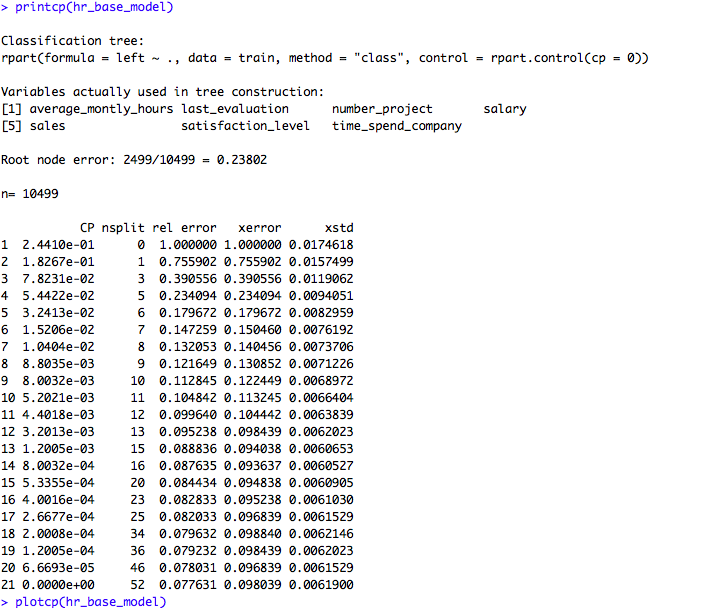
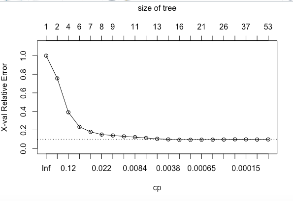
printcp(hr_base_model)
plotcp(hr_base_model)

If we look at the summary of hr_base_model in the above code snippet, it shows the statistics for all splits. The printcp and plotcp functions provide the cross-validation error for each nsplit and can be used to prune the tree. The one with least cross-validated error (xerror) is the optimal value of CP given by the printcp() function. The use of this plot is described in the post-pruning section.

Next, the accuracy of the model is computed and stored in a variable base_accuracy.

# Compute the accuracy of the pruned tree
test$pred <- predict(hr_base_model, test, type = "class")
base_accuracy <- mean(test$pred == test$left)

There are chances that the tree might overfit the dataset. In such cases, we can go with pruning the tree. Pruning is mostly done to reduce the chances of overfitting the tree to the training data and reduce the overall complexity of the tree. 

There are two types of pruning: pre-pruning and post-pruning.

Prepruning

Prepruning is also known as early stopping criteria. As the name suggests, the criteria are set as parameter values while building the rpart model. Below are some of the pre-pruning criteria that can be used. The tree stops growing when it meets any of these pre-pruning criteria, or it discovers the pure classes.

• maxdepth: This parameter is used to set the maximum depth of a tree. Depth is the length of the longest path from a Root node to a Leaf node. Setting this parameter will stop growing the tree when the depth is equal the value set for maxdepth.

• minsplit: It is the minimum number of records that must exist in a node for a split to happen or be attempted. For example, we set minimum records in a split to be 5; then, a node can be further split for achieving purity when the number of records in each split node is more than 5.

• minbucket: It is the minimum number of records that can be present in a Terminal node. For example, we set the minimum records in a node to 5, meaning that every Terminal/Leaf node should have at least five records. We should also take care of not overfitting the model by specifying this parameter. If it is set to a too-small value, like 1, we may run the risk of overfitting our model.

# Grow a tree with minsplit of 100 and max depth of 8
hr_model_preprun <- rpart(left ~ ., data = train, method = "class", 
                   control = rpart.control(cp = 0, maxdepth = 8,minsplit = 100))
# Compute the accuracy of the pruned tree
test$pred <- predict(hr_model_preprun, test, type = "class")
accuracy_preprun <- mean(test$pred == test$left)

Postpruning

The idea here is to allow the decision tree to grow fully and observe the CP value. Next, we prune/cut the tree with the optimal CP value as the parameter as shown in below code:

#Postpruning
# Prune the hr_base_model based on the optimal cp value
hr_model_pruned <- prune(hr_base_model, cp = 0.0084 )
# Compute the accuracy of the pruned tree
test$pred <- predict(hr_model_pruned, test, type = "class")
accuracy_postprun <- mean(test$pred == test$left)
data.frame(base_accuracy, accuracy_preprun, accuracy_postprun)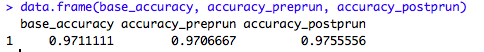

The accuracy of the model on the test data is better when the tree is pruned, which means that the pruned decision tree model generalizes well and is more suited for a production environment. However, there are also other factors that can influence decision tree model creation, such as building a tree on an unbalanced class. These factors were not accounted for in this demonstration but it's very important for them to be examined during a live model formulation.